Water density and viscosity

The density (\(\rho\), kg m-3) and viscosity (\(\mu\), Pa s) of water are required inputs to the calculation of productivity and other calculations within pyrealm. Both quantities vary with temperature and atmospheric pressure, although the variation with pressure is very small. However, the behaviour of water viscosity and density with temperature is highly complex and algorithms for calculating them differ very widely in the level of precision that they aim to achieve.

The pyrealm package provides a number of implementations for both quantities. This includes very high precision implementations but these are expensive to calculate and may be far more precise than is really warranted, given uncertainty in forcing variables or the accuracy required for day to day usage. This page reviews the available methods and shows the relative precision and computational complexity of alternative methods.

Note

The methods implemented in pyrealm are a sample of a wide range of different implementations of varying complexity. They are not intended to be an exhaustive survey, just to provide reasonable approaches of varying complexity.

Water density

The pyrealm.core.water module provides the following alternative methods for calculating water density:

kell (calculate_density_h2o_kell(), (Kell, 1975)),
jones_harris_eq6 (calculate_density_h2o_jones_harris_eq6(), (Jones and Harris, 1992)),
jones_harris_eq8 (calculate_density_h2o_jones_harris_eq8(), (Jones and Harris, 1992)),
chen (calculate_density_h2o_chen(), Chen et al. (2008)),
fisher (calculate_density_h2o_fisher(), Fisher and Dial Jr (1975))

The first two of these implementations (kell, jones_harris_eq6) do not correct for the effects of atmospheric pressure - although the functions require patm as inputs, these values are not then used in the calculation.

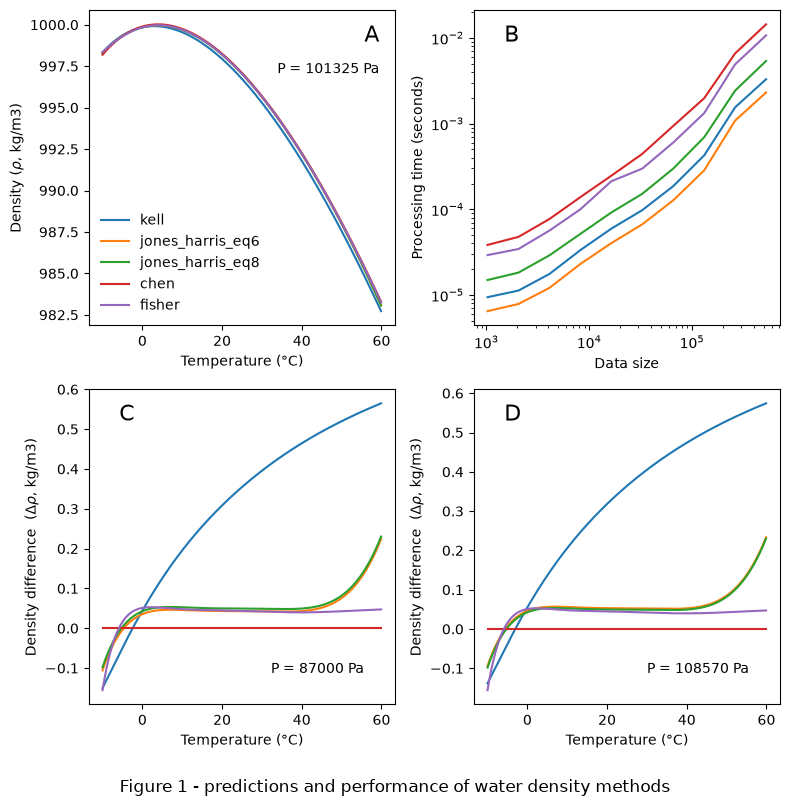
../_images/87331810c48744f7f1c71f610361d014401c695de0a876d32b7cf39c10d59a29.png

Figure 1A shows the predicted variation in density for each of the methods. Figure 1B shows the computational performance of each method: the most complex method (chen) is an order of magnitude slower than the fastest method (jones_harris_eq6). Figure 1C and 1D show the differences between predicted \(\rho\), relative to the chen method: the differences in predicted \(\rho\) are small, particularly in the temperature range of 0-40°C. Comparing Figure 1C and 1D, differences in predicted \(\rho\) due to atmospheric pressure are extremely small and accounting for them is unlikely to be useful.

Water viscosity

The pyrealm.core.water module provides the following methods for calculating water viscosity.

vogel (calculate_viscosity_h2o_vogel())
viswanath_natarajan (calculate_viscosity_h2o_viswanath_natarajan())
girifalco (calculate_viscosity_h2o_girifalco())
reid (calculate_viscosity_h2o_reid())
daubert_danner (calculate_viscosity_h2o_daubert_danner())
huber (calculate_viscosity_h2o_huber())

Only the last of these (huber) corrects for the effect of atmospheric pressure. Again, all the functions require patm as inputs, but these values are only used by the huber method.

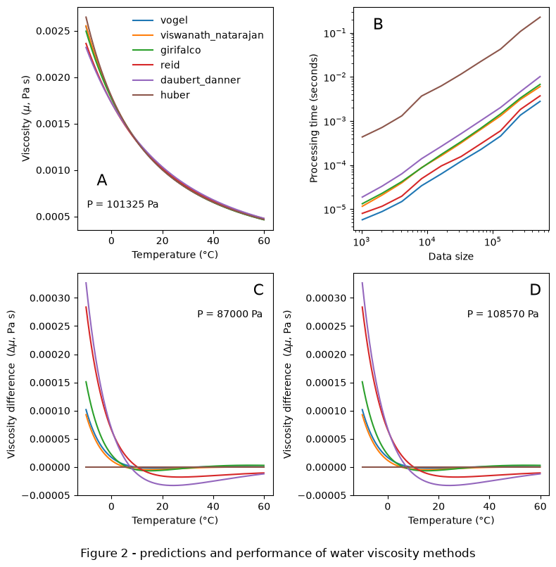
../_images/1ecc868ed64da3b35659aff6074a66e631fb8d072ad29cd6282559ab107efea6.png

Figure 2A shows the predicted variation in viscosity with temperature. Figure 2B shows that the most complex method (huber) is roughly two orders of magnitude slower than the fastest method (vogel). The differences in predicted viscosity from the most complex method (Figure 2C,D) are again very small, particularly within reasonable temperatures (~0-60°C), and the effects of atmospheric pressure are tiny (compare Figure 2C,D).

Effect on GPP predictions

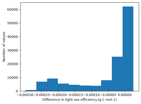
The code below fits the standard PModel to example data using the most complex and then most efficient implementations. The following plot then shows the difference in estimated light use efficiency between the two models. The conditions in the example data cover a wide range of possible environmental conditions and the absolute difference in light use efficiency arising from using the different implementations is extremely small.

# Load an example dataset containing the forcing variables.
data_path = resources.files("pyrealm_build_data.rpmodel") / "pmodel_global.nc"
ds = xarray.load_dataset(data_path)

# Extract the six variables for the two months
temp = ds["temp"]
co2 = ds["CO2"]
elev = ds["elevation"]
vpd = ds["VPD"]
fapar = np.array([1.0])
ppfd = np.array([1.0])

# Convert elevation to atmospheric pressure
patm = calculate_patm(elev)

# Mask out temperature values below -25°C
temp = temp.where(temp >= -25)

# Clip VPD to force negative VPD to be zero
vpd = np.clip(vpd, 0, np.inf)

# Calculate the photosynthetic environment using different viscosity calculations.
env_high_precision = PModelEnvironment(
    tc=temp,
    co2=co2,
    patm=patm,
    vpd=vpd,
    fapar=fapar,
    ppfd=ppfd,
    core_const=CoreConst(water_density_method="chen", water_viscosity_method="huber"),
)
env_lower_precision = PModelEnvironment(
    tc=temp,
    co2=co2,
    patm=patm,
    vpd=vpd,
    fapar=fapar,
    ppfd=ppfd,
    core_const=CoreConst(
        water_density_method="jones_harris_eq6", water_viscosity_method="vogel"
    ),
)

# Run the P model
model_higher_precision = PModel(env_high_precision)
model_lower_precision = PModel(env_lower_precision)

# Calculate and plot the difference
diff = model_higher_precision.gpp - model_lower_precision.gpp
plt.hist(diff.flatten())
plt.ylabel("Number of values")
_ = plt.xlabel("Difference in light use efficiency (g C mol-1)")

/home/docs/checkouts/readthedocs.org/user_builds/pyrealm/checkouts/latest/pyrealm/pmodel/pmodel.py:481: UserWarning: 
    Pyrealm 2.0.0 uses a new default for the quantum yield of photosynthesis (phi0=1/8).
    You may need to change settings to duplicate results from pyrealm 1.0.0.
            
  warn(

../_images/4a0447f48b9c2c4016a39d38d5999cc4327a3adc52a778de99f0be3f9ed444a6.png