The SPLASH model
Run this notebook
Read the guide on setting up your computer to run Jupyter notebooks
Download
this notebookas a Jupyter notebook.
The splash module provides a new implementation of the SPLASH v1.0 model
for estimating soil moisture, actual evapotranspiration (AET) and surface water
runoff. The model takes an initial estimate of soil moisture and then uses time series
of precipitation, temperature and incoming radiation to estimate how the daily water
balance changes with precipitation , condensation and AET. The water balance equation
is:
That is, the current soil moisture (mm, \(W_{n[t]}\)) is:
The soil moisture from yesterday (mm, \(W_{n[t-1]}\)),
plus the precipitation for today (mm d-1, \(P_{[t]}\)),
plus the condensation for today (mm d-1, \(C_{[t]}\)),
minus the expected evapotranspiration during the day (mm d-1, \(\textrm{AET}_{[t]}\)).
Calculations of AET and condensation are affected by the soil moisture, temperature and downwelling solar radiation at the site: this requires that the elevation and latitude of the site are known.
The calculated value of \(W_{n[t]}\) is then capped at the maximum soil moisture capacity (\(W_m\)) of the site, with excess water allocated to surface water runoff: if \(W_{n[t]} > W_m\), then \(W_{n[t]} = W_m, R_{[t]} = W_{n[t]} - W_m\). The maximum soil moisture capacity defaults to the original SPLASH value of 150 mm, but this can be set on a per site basis.
Solar radiation
The original implementation of the SPLASH v1 model (Davis et al., 2017) was designed to work with datasets that provided cloud cover data. The model calculated the solar radiation reaching the top of the atmosphere and then calculated how much of the radiation reached the ground, given the cloud cover and site elevation.
The more recent SPLASH v2 model (Sandoval et al., 2024) updated the solar flux calculations to use estimates of shortwave downwelling radiation on the ground. This is now commonly provided with remotely sensed climate data and is also common in site-based data such as FluxNET.
The implementation in pyrealm supports both of these options - you can provide either
sunshine fraction (1 - cloud cover) or shortwave radiation in W m-2.
Important
The SPLASH v2 model (Sandoval et al., 2024) includes a large number of other extensions
to improve the calculation of soil moisture, including the effects of slope and aspect
and snow on shortwave reflection (the albedo) and a much more detailed soil capacity
model. Only the calculation of daily solar fluxes from shortwave radiation has been
added in pyrealm.
Example 1: Gridded data using sunshine fraction
The data below provides a 2 year daily time series of precipitation, temperature and sunshine fraction (1 - cloud cover) for 0.5° resolution grid cells in a 10° by 10° block of the North Western USA. It also provides the mean elevation of those cells.
from importlib import resources
import numpy as np
import xarray
import pandas as pd
from matplotlib import pyplot as plt
import matplotlib.dates as mdates

from pyrealm.splash.splash import SplashModel
from pyrealm.core.calendar import Calendar
from pyrealm.core.datasets import get_pyrealm_data

# Load gridded data
dpath = get_pyrealm_data("splash/data/splash_nw_us_grid_data.nc")
data = xarray.load_dataset(dpath)

# Define three sites for showing time series
sites = xarray.Dataset(
    data_vars=dict(
        lon=(["site_id"], [-122.419, -119.538, -116.933]),
        lat=(["site_id"], [37.775, 37.865, 36.532]),
    ),
    coords=dict(site_id=(["San Francisco", "Yosemite", "Death Valley"])),
)

data
<xarray.Dataset> Size: 5MB
Dimensions:  (lat: 20, lon: 20, time: 731)
Coordinates:
  * lat      (lat) float64 160B 36.25 36.75 37.25 37.75 ... 44.75 45.25 45.75
  * lon      (lon) float64 160B -124.8 -124.2 -123.8 ... -116.2 -115.8 -115.2
  * time     (time) datetime64[ns] 6kB 2000-01-01 2000-01-02 ... 2001-12-31
Data variables:
    elev     (lat, lon) float32 2kB nan nan nan ... 1.663e+03 1.679e+03
    tmp      (time, lat, lon) float32 1MB nan nan nan ... -0.6357 -2.712 -4.778
    pre      (time, lat, lon) float64 2MB nan nan nan nan ... 0.0 0.0 0.0 0.0
sf (time, lat, lon) float32 1MB nan nan nan nan ... 0.187 0.2 0.2The plot below shows the elevation for the example data area, along with the locations of three sites that will be used to compare SPLASH outputs.
# Get the latitude and longitude extents
extent = (
    data["lon"].min(),
    data["lon"].max(),
    data["lat"].min(),
    data["lat"].max(),
)
# Plot the elevation
plt.imshow(data["elev"], extent=extent, origin="lower")

# Add three sites
plt.plot(sites["lon"].data, sites["lat"].data, "ro")
for x, y, site_name in zip(sites["lon"], sites["lat"], sites["site_id"]):
    plt.text(x, y + 0.2, site_name.data, color="red", ha="center", va="bottom")
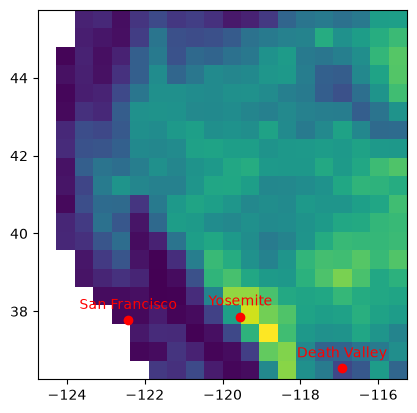
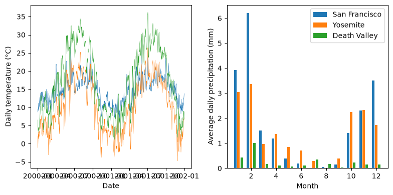
The three sites capture wetter coastal conditions with milder temperatures (San Francisco), intermediate rainfall with colder temperatures (Yosemite) and arid conditions with extreme temperatures (Death Valley).
# Get three sites to show time series for locations
site_data = data.sel(sites, method="nearest")

fig, (ax1, ax2) = plt.subplots(1, 2, figsize=(8, 4))

for idx, site_name in enumerate(site_data["site_id"].data):
    ax1.plot(
        site_data["time"].data,
        site_data["tmp"].data[:, idx],
        linewidth=0.4,
        label=site_name,
    )

ax1.set_xlabel("Date")
ax1.set_ylabel("Daily temperature (°C)")

# Calculate the average daily precipitation within months for each site
month_length = site_data.time.dt.days_in_month
weights = month_length.groupby("time.month") / month_length.groupby("time.month").sum()
ave_daily_pre = (site_data["pre"] * weights).groupby("time.month").sum(dim="time")

for offset, site_name in zip([-1, 0, 1], site_data["site_id"].data):
    ax2.bar(
        ave_daily_pre["month"] + offset * 0.25,
        ave_daily_pre.sel(site_id=site_name),
        width=0.2,
        label=site_name,
    )

ax2.set_xlabel("Month")
ax2.set_ylabel("Average daily precipitation (mm)")
ax2.legend()

plt.tight_layout()
Running the splash model
Initialising a SplashModel
Before calculating water balances, you need to create a
SplashModel. This takes the site data and runs all of
the solar and evaporative calculations for the time series - none of these calculations
rely on the soil moisture and so are calculated once when the SplashModel is created.
# Fit the model
splash = SplashModel(
    latitude=data.lat,
    elevation=data.elev,
    dates=Calendar(data.time),
    sunshine_fraction=data.sf,
    temperature=data.tmp,
    precipitation=data.pre,
)
The data for the incoming radiation (sunshine fraction in this example), temperature and precipitation are arrays providing values along through time. In this case the arrays are 3D, providing data on a latitude and longitude grid, but input data could be 1D (a single site) or 2D (a set of sites).
Note that latitude only varies along the latitude axis and elevation is constant through
time. You need to take care to ensure that array dimensions along the different axes
are compatible. In this example, the data is from an xarray
dataset, and pyrealm uses the extra dimension information in the dataset to align the
data.
Estimating initial soil moisture
To calculate daily water balances, you need initial values for the soil moisture. This
data is rarely available and so the
estimate_initial_soil_moisture() can be used to
estimate those values.
The method requires that the input data provides at least one full year of data. It works by assuming that soil moisture change is a stationary process on an annual time scale: the initial soil moisture should be the same as the soil moisture at the end of the year, given the observed annual data.
init_soil_moisture = splash.estimate_initial_soil_moisture()
This method estimates the soil moisture over a year, starting with an initial guess at
the soil moisture at the start of the year. It then compares the predicted soil
moisture at the start and the end of the year and uses the difference between the two to
update the initial guess and re-run the year. This iteration should converge on an
initial value for the start of the year, that leads to a very similar prediction at the
end of the year. This convergence can sometime fail: see the
estimate_initial_soil_moisture() documentation
for details on how to fine tune the convergence process.
Calculating water balance
The SplashModel provides the
estimate_daily_water_balance() method. This
takes the index of one of the days in the observed data and the soil moisture from the
previous day and uses the equation above to calculate the new soil moisture. The code
below uses the method to calculate the soil moisture for the first day, given the
initial soil moisture estimates.
Note
The estimate_daily_water_balance method only calculates a single iteration of the
water balance across sites. Usually you would use calculate_soil_moisture (see below)
to run the calculations over the whole time series, but the method is used here to show
how the process works for the first step.
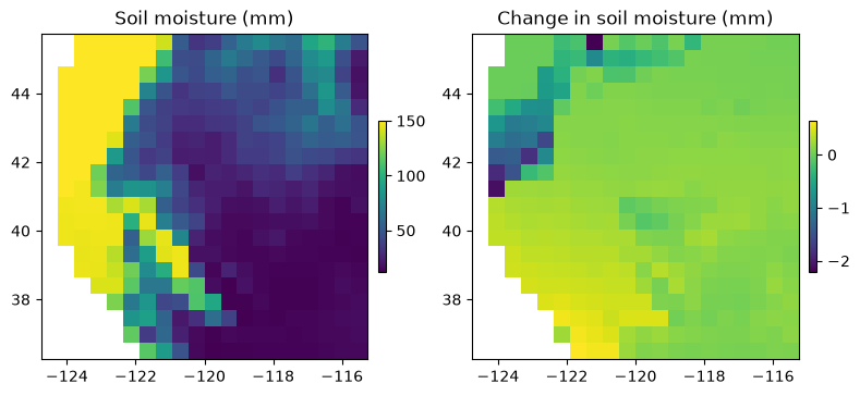
The plots show the soil moisture for the first day, along with the changes in soil moisture from the initial estimates (the ‘previous day’). Note the saturated soil moisture of 150mm near the coast and in the mountains.
# Calculate the water balance equation for the first day from the initial soil
#  moisture estimates.
aet, wn, ro = splash.estimate_daily_water_balance(
    previous_soil_moisture=init_soil_moisture, day_index=0
)

# Plot the calculated soil moisture and change from previous values.
fig, (ax1, ax2) = plt.subplots(1, 2, figsize=(8, 4))
im_val = ax1.imshow(wn, extent=extent, origin="lower")
plt.colorbar(im_val, fraction=0.022, pad=0.03)
ax1.set_title("Soil moisture (mm)")

diff_val = ax2.imshow(init_soil_moisture - wn, extent=extent, origin="lower")
plt.colorbar(diff_val, fraction=0.022, pad=0.03)
ax2.set_title("Change in soil moisture (mm)")

plt.tight_layout()
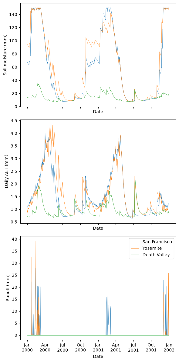
The calculate_soil_moisture() method iterates
the daily estimation across all of the dates in the input data from initial soil
moisture estimates. It returns a set of time series of soil moisture, runoff and AET for
all sites.
aet_out, wn_out, ro_out = splash.calculate_soil_moisture(
    initial_soil_moisture=init_soil_moisture
)
The plots below show the resulting soil moisture and a time series for the three
# Add the outputs to the xarray to select the three sites easily.
data["aet"] = xarray.DataArray(aet_out, dims=("time", "lat", "lon"))
data["wn"] = xarray.DataArray(wn_out, dims=("time", "lat", "lon"))
data["ro"] = xarray.DataArray(ro_out, dims=("time", "lat", "lon"))
site_data = data.sel(sites, method="nearest")

fig, axes = plt.subplots(3, 1, figsize=(6, 12), sharex=True)

for ax, var_name, ax_label in zip(
    axes, ["wn", "aet", "ro"], ["Soil moisture (mm)", "Daily AET (mm)", "Runoff (mm)"]
):
    for idx, site_name in enumerate(site_data["site_id"].data):
        ax.plot(
            site_data["time"].data,
            site_data[var_name].data[:, idx],
            linewidth=0.5,
            label=site_name,
        )
    ax.set_xlabel("Date")
    ax.set_ylabel(ax_label)

    # Format date axis
    myFmt = mdates.DateFormatter("%b\n%Y")
    ax.xaxis.set_major_formatter(myFmt)


plt.legend()
plt.tight_layout()
Example 2: Site data using shortwave radiation
This example uses data from the Bourne SNOTEL site. The dataset provides eight years of data for the site and provides solar radiation as shortwave downwelling radiation, rather than sunshine fraction.
Important
Note that this site is cold and snowy. Unlike the SPLASH v2 model, the SPLASH v1 model used here does not capture snow dynamics and the effect of snow on shortwave albedo.
# Load site data
dpath = get_pyrealm_data("rsplash/rsplash_Bourne_inputs.csv")
bourne = pd.read_csv(dpath)

bourne.head()
| Unnamed: 0 | date | P | Ta | sw_in | swe | sm | elev | lat | |
|---|---|---|---|---|---|---|---|---|---|
| 0 | 1 | 2008-01-01 | 0.00 | -9.444444 | 71.423998 | 200.90 | 82.908 | 1783.08 | 44.83 |
| 1 | 2 | 2008-01-02 | 0.00 | -6.111111 | 62.208001 | 200.90 | 85.554 | 1783.08 | 44.83 |
| 2 | 3 | 2008-01-03 | 2.54 | -2.777778 | 54.745597 | 203.35 | 83.104 | 1783.08 | 44.83 |
| 3 | 4 | 2008-01-04 | 7.62 | -2.222222 | 26.790399 | 205.80 | 85.162 | 1783.08 | 44.83 |
| 4 | 5 | 2008-01-05 | 7.62 | -5.000000 | 31.449600 | 213.15 | 84.672 | 1783.08 | 44.83 |
# Generate the Calendar object from the dates
days = bourne["date"].to_numpy().astype("datetime64[D]")
calendar = Calendar(days)

# Initialise the model
bourne_splash = SplashModel(
    latitude=bourne["lat"].to_numpy(),
    elevation=bourne["elev"].to_numpy(),
    temperature=bourne["Ta"].to_numpy(),
    precipitation=bourne["P"].to_numpy(),
    shortwave_radiation=bourne["sw_in"].to_numpy(),
    dates=calendar,
)

# Calculate initial estimates of soil moisture
init_soil_moisture = bourne_splash.estimate_initial_soil_moisture()

# Calculate soil moisture
aet_out, wn_out, ro_out = bourne_splash.calculate_soil_moisture(init_soil_moisture)
/home/docs/checkouts/readthedocs.org/user_builds/pyrealm/checkouts/latest/pyrealm/core/bounds.py:157: UserWarning: Variable 'shortwave_radiation' is not configured in the bounds checker. No bounds checking performed.
  warn(
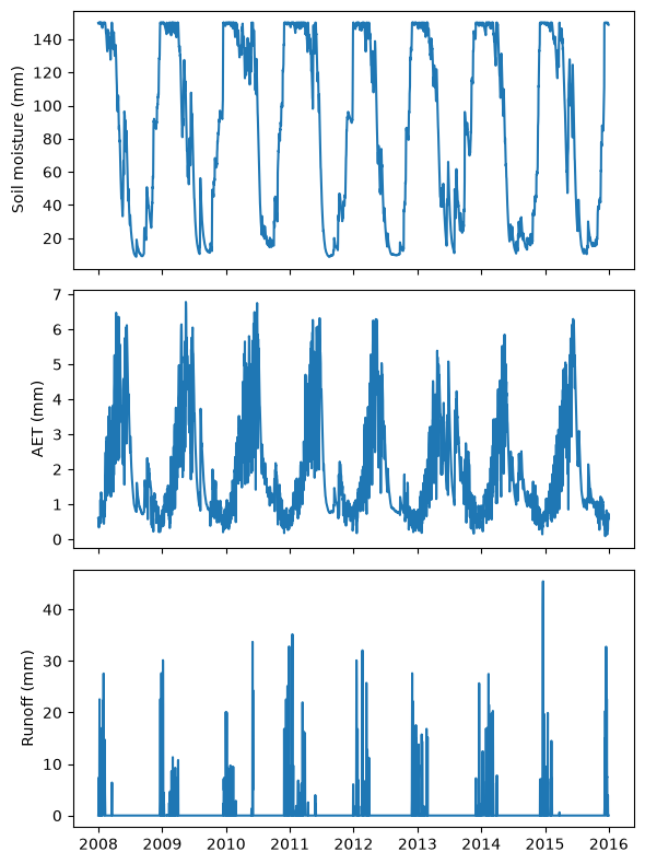
The plots below show the predicted values for the site.
fig, (ax1, ax2, ax3) = plt.subplots(nrows=3, sharex=True, figsize=(6, 8))

ax1.plot(days, wn_out)
ax1.set_ylabel("Soil moisture (mm)")
ax2.plot(days, aet_out)
ax2.set_ylabel("AET (mm)")
ax3.plot(days, ro_out)
ax3.set_ylabel("Runoff (mm)")

plt.tight_layout()