C3 / C4 Competition

Run this notebook

• Read the guide on setting up your computer to run Jupyter notebooks

• Download this notebook as a Jupyter notebook.

Compared to C3 plants, plants using the C4 photosynthetic pathway:

• cope well in arid areas, operating with lower stomatal conductance and lower leaf internal CO2 than C3 plants,

• are strongly favoured in lower atmospheric CO2 concentrations, and

• do not experience significant photorespiration costs.

This gives C4 plants a substantial competitive advantage in warm, dry and low CO2 environments. The C3C4Competition class provides an implementation of a model (Lavergne et al., 2022) that estimates the expected fraction of GPP from C4 plants. It uses predictions of GPP from the PModel assuming communities consisting solely of C3 or C4 plants to calculate the expected fraction of C4 plants in the community and the contributions to GPP from C3 and C4 plants at each site.

Step 1: Proportional GPP advantage

The first step is to calculate the proportional advantage in gross primary productivity (GPP) of C4 over C3 plants (\(A_4\)) in the study locations.

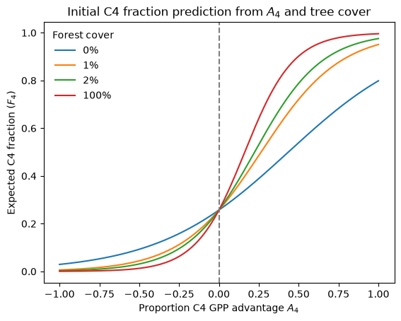
Step 2: Convert GPP advantage to the fraction of C4 plants

A statistical model is then used to convert the proportional C4 GPP advantage to the expected C4 fraction (\(F_4\)) in a community (see C3C4Competition for details). This model includes a correction term for the estimated percentage tree cover and the plot below shows how \(F_4\) changes with \(A_4\), given differing estimates of tree cover.

Show code cell source

Hide code cell source

import numpy as np
import matplotlib.pyplot as plt
from matplotlib.lines import Line2D

from pyrealm.pmodel.pmodel import PModel
from pyrealm.pmodel import (
    PModelEnvironment,
    CarbonIsotopes,
    C3C4Competition,
    convert_gpp_advantage_to_c4_fraction,
    calculate_tree_proportion,
)

# Generate 2D arrays for combinations of GPP advantage and tree cover
gpp_adv_c4_1d = (np.linspace(-1, 1, 201),)
treecover_1d = np.array([0, 1, 2, 100])
gpp_adv_c4_2d, treecover_2d = np.meshgrid(gpp_adv_c4_1d, treecover_1d)

# Get the conversion
frac_c4 = convert_gpp_advantage_to_c4_fraction(gpp_adv_c4_2d, treecover_2d)

# Plot the results
for idx, lev in enumerate(treecover_1d):
    plt.plot(gpp_adv_c4_2d[idx, :], frac_c4[idx, :], label=f"{int(lev)}%")

plt.legend(title="Forest cover", frameon=False)
plt.title(r"Initial C4 fraction prediction from $A_4$ and tree cover")
plt.xlabel("Proportion C4 GPP advantage $A_4$")
plt.ylabel("Expected C4 fraction ($F_4$)")
plt.axvline(0, ls="--", c="grey")
plt.show()

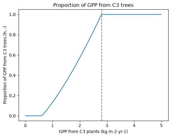
Step 3: Account for shading by C3 trees

The fraction of C4 plants can be reduced below expectations simply from relative GPP advantage by shading from C3 trees. A statistical model is used to predict the proportion of GPP expected from C3 trees (\(h\)) and this is used to discount \(F_4 = F_4 (1-h)\).

The plot below shows how \(h\) varies with the expected GPP from C3 plants alone. The dashed line shows the C3 GPP estimate above which canopy closure leads to complete shading of C4 plants.

Show code cell source

Hide code cell source

# Just use the competition model to predict h across a GPP gradient
gpp_c3_kg = np.linspace(0, 5, 101)
prop_trees = calculate_tree_proportion(gpp_c3_kg)
plt.plot(gpp_c3_kg, prop_trees)
plt.axvline(2.8, ls="--", c="grey")

plt.title("Proportion of GPP from C3 trees")
plt.xlabel("GPP from C3 plants (kg m-2 yr-1)")
plt.ylabel("Proportion of GPP from C3 trees (h, -)")
plt.show()

Step 4: Filtering cold areas and cropland

The last steps are to set \(F_4 = 0\) for locations where the mean temperature of the coldest month is below a threshold for the persistence of C4 plants (below_t_min) and then to remove predictions for croplands (cropland), where the C4 fraction is driven by agricultural management.

Predicted GPP and expected isotopic signatures

The resulting model predicts the fraction of GPP from C4 and hence the actual contributions to total GPP from the C3 and C4 pathways. In addition, the model can be used to generate the expected isotopic signatures resulting from the predicted fractions of C3 and C4 plants.

Worked example

The code below shows the various stages of the model for example annual GPP predictions for C3 plants and C4 plants alone across a temperature gradient with an estimated tree cover of 0.5.

Code

# Use a simple temperature sequence to generate a range of optimal chi values
n_pts = 51
tc_1d = np.linspace(-10, 45, n_pts)

# Fit C3 and C4 P models
env = PModelEnvironment(tc=tc_1d, patm=101325, co2=400, vpd=1000, ppfd=450, fapar=0.9)

mod_c3 = PModel(env, method_optchi="prentice14")

mod_c4 = PModel(env, method_optchi="c4")

# Competition, using annual GPP from µgC m2 s to g m2 yr
gpp_c3_annual = mod_c3.gpp * (60 * 60 * 24 * 365) * 1e-6
gpp_c4_annual = mod_c4.gpp * (60 * 60 * 24 * 365) * 1e-6

# Fit the competition model
comp = C3C4Competition(
    gpp_c3=gpp_c3_annual,
    gpp_c4=gpp_c4_annual,
    treecover=0.5,
    below_t_min=False,
    cropland=False,
)

# Calculate step by step components of model
frac_c4_step2 = convert_gpp_advantage_to_c4_fraction(comp.gpp_adv_c4, 0.5)
prop_trees = calculate_tree_proportion(gppc3=gpp_c3_annual / 1000)
frac_c4_step3 = frac_c4_step2 * (1 - prop_trees)

# Generate isotopic predictions
isotope_c3 = CarbonIsotopes(mod_c3, d13CO2=-8.4, D14CO2=19.2)
isotope_c4 = CarbonIsotopes(mod_c4, d13CO2=-8.4, D14CO2=19.2)

comp.estimate_isotopic_discrimination(
    d13CO2=-8.4,
    Delta13C_C3_alone=isotope_c3.Delta13C,
    Delta13C_C4_alone=isotope_c4.Delta13C,
)

comp.summarize()

C3C4Competition(shape=(51,))
Attr               Mean     Min      Max    NaN  Units
--------------  -------  ------  -------  -----  -----------
frac_c4            0.06    0        0.87      0  -
gpp_c3_contrib  3516.9   129.61  5028.95      0  gC m-2 yr-1
gpp_c4_contrib   302.39    0     3865.25      0  gC m-2 yr-1
Delta13C_C3       16.8     2.96    22.49      0  permil
Delta13C_C4        0.06    0        0.52      0  permil
d13C_C3          -24.77  -30.21   -11.32      0  permil
d13C_C4           -8.46   -8.92    -8.4       0  permil

/home/docs/checkouts/readthedocs.org/user_builds/pyrealm/checkouts/latest/pyrealm/pmodel/pmodel.py:481: UserWarning: 
    Pyrealm 2.0.0 uses a new default for the quantum yield of photosynthesis (phi0=1/8).
    You may need to change settings to duplicate results from pyrealm 1.0.0.
            
  warn(
/home/docs/checkouts/readthedocs.org/user_builds/pyrealm/checkouts/latest/pyrealm/core/experimental.py:72: ExperimentalFeatureWarning: 'Be aware that C3C4Competition is an experimental feature of pyrealm and the implementation and API may change within major versions.'
  warn(qualname, ExperimentalFeatureWarning)

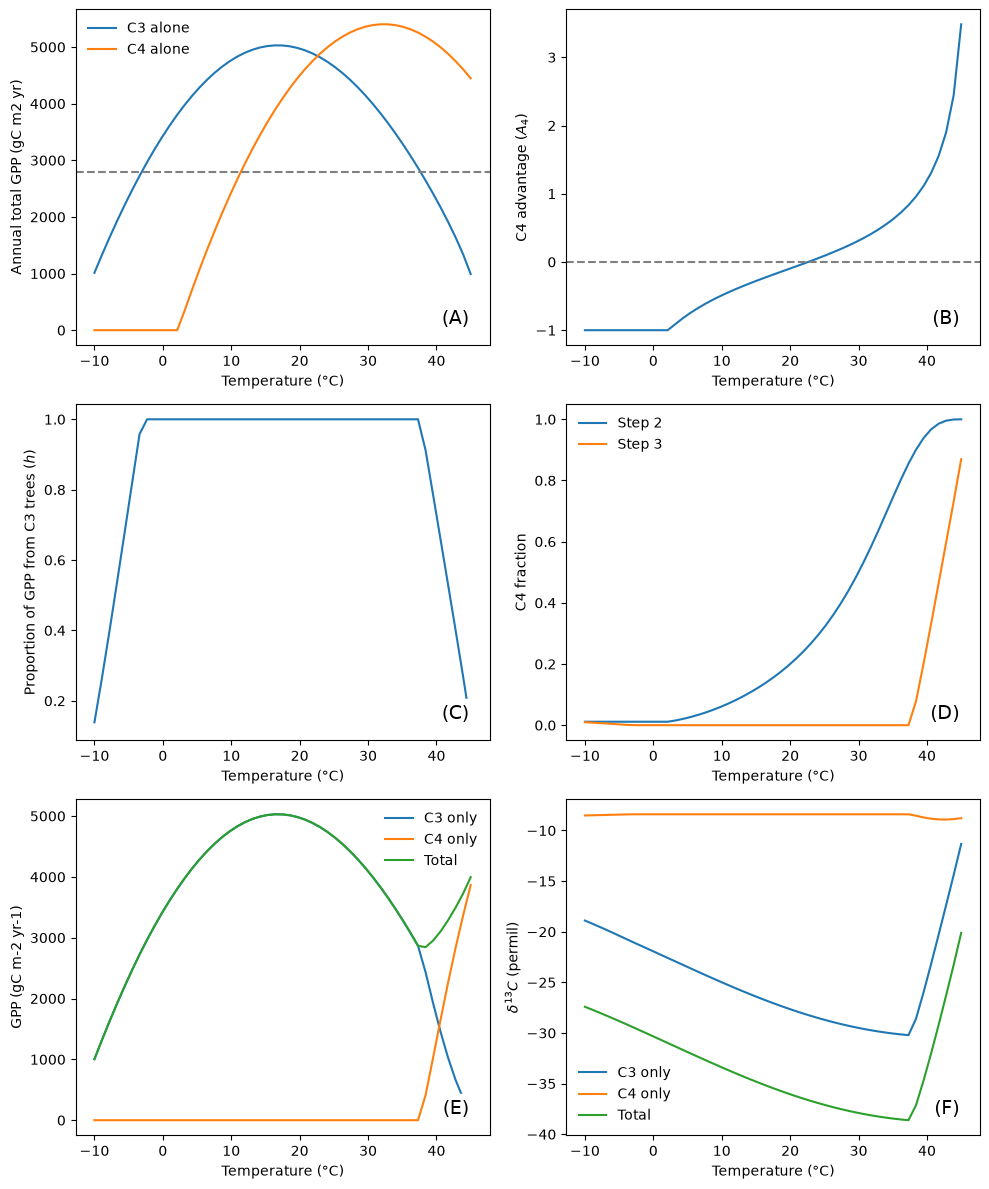
Figures

The plots below then show the various stages of the model prediction.

Panel A

GPP predictions from the P model across a temperature gradient for C3 or C4 plants alone. The horizontal dashed line shows the canopy closure threshold for C3 plants (see Step 3).

Panel B

The relative GPP advantage of C4 over C3 photosynthesis across the temperature gradient.

Panel C

The proportion of GPP from C3 trees across the temperature gradient. Between roughly 5°C and 30°C, canopy closure is predicted to exclude C4 plants, even where they have a GPP advantage (Panel B, > 22°C).

Panel D

Predicted \(F_4\) across the temperature gradient, showing the prediction purely from relative advantage and treecover (Step 2) and then accounting for the impact of C3 tree canopy closure (Step 3),

Panel E

The predicted contributions of plants using the C3 and C4 pathways to the total expected GPP

Panel F

The contributions of plants using the C3 and C4 pathways to predicted \(\delta\ce{^{13}C}\) .

Show code cell source

Hide code cell source

# Generate the plots
fig, ((ax1, ax2), (ax3, ax4), (ax5, ax6)) = plt.subplots(3, 2, figsize=(10, 12))

# GPP predictions
ax1.plot(tc_1d, gpp_c3_annual, label="C3 alone")
ax1.plot(tc_1d, gpp_c4_annual, label="C4 alone")
# ax1.set_title(r'Variation in GPP with temperature')
ax1.set_xlabel("Temperature (°C)")
ax1.set_ylabel(r"Annual total GPP (gC m2 yr)")
ax1.axhline(2800, ls="--", c="grey")  # canopy closure
ax1.legend(frameon=False)

# C4 Advantage predictions
ax2.plot(tc_1d, comp.gpp_adv_c4)
# ax2.set_title(r'Proportional GPP advantage of C4 over C3 ($A_4$)')
ax2.set_xlabel("Temperature (°C)")
ax2.set_ylabel(r"C4 advantage ($A_4$)")
ax2.axhline(0, ls="--", c="grey")

# Proportion of GPP from C3 trees
ax3.plot(tc_1d, prop_trees)
# ax3.set_title(r'Proportion of GPP from C3 trees ($h$)')
ax3.set_xlabel("Temperature (°C)")
ax3.set_ylabel(r"Proportion of GPP from C3 trees ($h$)")

# Expected C4 fraction by stage
ax4.plot(tc_1d, frac_c4_step2, label="Step 2")
ax4.plot(tc_1d, frac_c4_step3, label="Step 3")
# ax4.set_title(r'C4 fraction across the temperature gradient')
ax4.set_xlabel("Temperature (°C)")
ax4.set_ylabel(r"C4 fraction")
ax4.legend(frameon=False)

# GPP contributions of C4 and C4
ax5.plot(tc_1d, comp.gpp_c3_contrib, label="C3 only")
ax5.plot(tc_1d, comp.gpp_c4_contrib, label="C4 only")
ax5.plot(tc_1d, comp.gpp_c3_contrib + comp.gpp_c4_contrib, label="Total")
# ax4.set_title(r'C4 fraction across the temperature gradient')
ax5.set_xlabel("Temperature (°C)")
ax5.set_ylabel(r"GPP (gC m-2 yr-1)")
ax5.legend(frameon=False)

# d13C contributions of C4 and C4
ax6.plot(tc_1d, comp.d13C_C3, label="C3 only")
ax6.plot(tc_1d, comp.d13C_C4, label="C4 only")
ax6.plot(tc_1d, comp.d13C_C3 + comp.d13C_C4, label="Total")
# ax4.set_title(r'C4 fraction across the temperature gradient')
ax6.set_xlabel("Temperature (°C)")
ax6.set_ylabel(r"$\delta^{13}C$ (permil)")
ax6.legend(frameon=False)

# Add plot letters.
for letter, ax in zip(("A", "B", "C", "D", "E", "F"), (ax1, ax2, ax3, ax4, ax5, ax6)):

    ax.text(
        0.95,
        0.05,
        f"({letter})",
        horizontalalignment="right",
        verticalalignment="bottom",
        transform=ax.transAxes,
        size=14,
        backgroundcolor="w",
    )

plt.tight_layout()