The canopy model
Run this notebook
Read the guide on setting up your computer to run Jupyter notebooks
Download
this notebookas a Jupyter notebook.
Warning
This area of pyrealm is in active development and this notebook currently contains
notes and initial demonstration code.
The canopy module in pyrealm is used to calculate a vertically structured model of
leaf distribution for set of cohorts forming a plant community within an area. The
purpose of the canopy module is two-fold:
to calculate the vertical distribution of crown and leaf area, including the partitioning of canopy into discrete vertical layers, and
to estimate light capture through canopy layers.
This page describes the model of the vertical canopy structure and the light capture model is presented separately.
Vertically structured canopies
The simplest “big leaf” model of a canopy, represents the entire crown crown (\(A_c\)) of
an individual tree as a single flat disc at the top of the stem. However, in pyrealm
the canopy model uses the crown shape described in the crown model to
model how leaf area accumulates vertically through a community.
Community definition
To recap, a plant community consists of a number of individual stems that are growing together in a location with a known area. The individuals are grouped together into cohorts that are defined as:
a number of individuals,
with identical diameter at breast height (DBH, \(D\)),
of the same plant functional type (PFT),
and hence have the same stem allometry and crown model.
However, for the purposes of the canopy model, it is much simpler to consider the community as a collection of individual stems, some of which just happen to share identical properties.
Community projected crown area
Each individual stem in a community has an projected crown area that describes how the crown area of that stem accumulates with height (\(z\)) from the top of the tree to the ground. The form of that curve varies with the size and PFT of the stem. If we have a community with \(N_s\) individuals, then each stem \(i = 1, ..., N_s\) has a projected crown area function \(A_{p}(z)_i\).
If we take the sum across all individuals of this function at a height \(z\), we get the total community projected crown area across all individual stems at that same height:
To demonstrate this, the code below creates a plant community that contains 12 individual stems, grouped into 3 cohorts with different stem sizes and crown shapes.
# Create a flora
flora = Flora(
    name=["short", "tall"],
    h_max=[15, 30],
    m=[2, 2],
    n=[4, 3],
    f_g=[0, 0],
    ca_ratio=[380, 500],
)

# Create an id generator.
cid_generator = cohort_id_generator(mode="str")

# Define a simply community with three cohorts
cohorts = create_cohorts(
    flora=flora,
    cid_generator=cid_generator,
    dbh_value=np.array([0.1, 0.20, 0.5]),
    n_individuals=np.array([7, 3, 2]),
    pft_name=np.array(["short", "short", "tall"]),
)

# Get the stem allometries
allometry = StemAllometry(cohorts)
The total crown area of the individuals in each of the three cohorts is shown below:
allometry.crown_area
array([ 2.08, 6.07, 43.43])
The total crown area across the community is then the sum of those crown areas across all individuals:
total_crown_area = np.sum(allometry.crown_area * cohorts.n_individuals)
total_crown_area
np.float64(119.64076045289785)
So, the total community crown area is around 120 m2. The plot below shows how \(C_p(z)\) changes with height for this community from zero at the top of the canopy to around 120 m2 at ground level. The horizontal dashed lines show the stem heights of the individuals, where the crown area of each individual starts contributing to the community wide projected crown area.
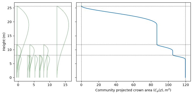
If the community is growing in an area greater than 120 m2, then the individuals can avoid overlapping any of their crown area. However, this is not possible if the community is growing in a smaller area, and some crown area must overlie other parts of the community, creating a vertical structure.
The canopy module implements the perfect plasticity approximation (PPA) model (Purves et al., 2008) to generate this structure. The PPA model assumes that all the individuals within the community are able to plastically arrange their crown at each height within the broader canopy of the community to fill available space. When the available horizontal space (\(A\)) is filled by the cumulative crown area across all individuals at a height \(z\), that canopy at that height forms a layer that is considered “full” (or “closed”). The remaining crown area below this layer then begins to accumulate into a new layer. This process repeats downward until the entire canopy structure is formed down to the ground.
To fit this model, we need to find the heights \(z^*_l\) at which the projected community crown area occupies multiples of the available area \(A\). This gives the heights at which each successive canopy layer closes for canopy layers \(l = 1, ..., l_m\). This is given as the equality:
An extra detail is that the canopy model includes a community-level canopy gap fraction (\(f_G\)) that captures the overall proportion of the canopy area that is left unfilled by canopy. This gap fraction, capturing processes such as crown shyness, describes the proportion of open sky visible from the forest floor. This term reduces the amount of \(A\) that can be occupied by crown area before a layer closes:
The values of \(z^*_l\) cannot be found analytically, so we use numerical methods to find values of \(z^*_l\) for \(l = 1,..., l_m\) that satisfy:
The total number of layers \(l_m\) in a canopy, where the final layer may not be fully closed, can be found given the total crown area across stems as:
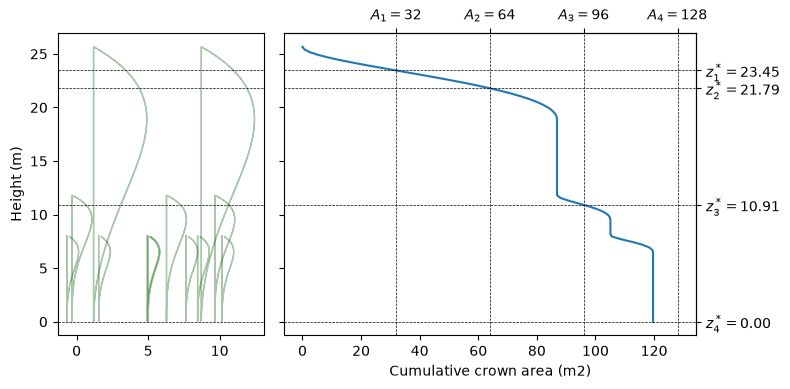
The community above has an available space \(A=32\;m^2\). If we fit the PPA model to this community we get the following heights:
# Fit the canopy model
canopy_ppa = Canopy(cohorts=cohorts, allometry=allometry, canopy_area=32, fit_ppa=True)
canopy_ppa.heights
array([23.45, 21.79, 10.91, 0. ])
We plot those layer heights below. The vertical dashed lines in the right hand plot show the values \(lA\) at which the cumulative space across layers forms closed layers: that is \(32 \times 1 = 32\), \(32 \times 2 = 64\), etc. . The horizontal dashed lines then show those calculated vertical heights. These are the canopy heights at which the vertical lines intersect the cumulative community projected crown area: where the total crown area across the individuals in the community fills each available layer.
We can look in detail at the how much crown area is in each layer from each individual. The canopy model object contains a crown profile which records the projected crown area at each height. Note how the bottom row - the total projected (i.e. cumulative) crown for the individuals in each cohort - matches the values above from the stem allometry calculations for the community.
canopy_ppa.crown_profile.projected_crown_area
array([[ 0.  ,  0.  , 16.  ],
       [ 0.  ,  0.  , 32.  ],
       [ 0.  ,  3.04, 43.43],
       [ 2.08,  6.07, 43.43]])
Those values are the projected crown areas of each individual within the cohorts: the accumulating crown area from the top of the canopy down to the ground. We can take the differences between vertical layers to give the actual amount of crown area in each layer for each individual within a cohort.
individual_crown_in_layer = np.diff(
    canopy_ppa.crown_profile.projected_crown_area, prepend=0, axis=0
)
individual_crown_in_layer
array([[ 0.  ,  0.  , 16.  ],
       [ 0.  ,  0.  , 16.  ],
       [ 0.  ,  3.04, 11.43],
       [ 2.08,  3.03,  0.  ]])
To bring those values back to the community model: since each value represents a cohort, we can multiply those values by the number of individuals and then find the row sums to show the total amount of crown area in each layer across all individuals and cohorts. As expected, the crown area in each layer matches the 32 m2 of available space, except for the last layer that is not completely filled.
np.sum(individual_crown_in_layer * cohorts.n_individuals.to_numpy(), axis=1)
array([32. , 32. , 32. , 23.64])
Crown and canopy gap fractions
The canopy and crown models are extended by providing two gap fractions:
The crown gap fraction (\(f_g\)) is described in detail in the crown model and captures how an individual tree crown may contain holes that displace leaf area further down into the canopy. Crown gaps do not push all the way down to the ground - they only allow light to penetrate more deeply into the crown.
The canopy gap fraction (\(f_G\)) is described above and captures how the canopy across the whole community may leave space unfilled in the canopy. Light passing through canopy gaps passes unimpeded from the top of the canopy down to the ground.
The code below alters the community and canopy model used above to include both crown and canopy gap fractions.
# Define a flora with PFTs that have crown gap fractions
gappy_flora = Flora(
    name=["short", "tall"],
    h_max=[15, 30],
    m=[2, 2],
    n=[4, 3],
    f_g=[0.1, 0.1],
    ca_ratio=[380, 500],
)

# Define a community with three cohorts of stems with gappy canopies
gappy_cohorts = create_cohorts(
    flora=gappy_flora,
    cid_generator=cid_generator,
    dbh_value=np.array([0.1, 0.20, 0.5]),
    n_individuals=np.array([7, 3, 2]),
    pft_name=np.array(["short", "short", "tall"]),
)
gappy_allometry = StemAllometry(gappy_cohorts)


gappy_canopy_ppa = Canopy(
    cohorts=gappy_cohorts,
    allometry=gappy_allometry,
    canopy_area=32,
    canopy_gap_fraction=1 / 8,
    fit_ppa=True,
)
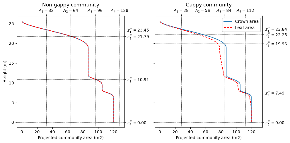
The plots below show the cumulative projected leaf and crown areas across the individuals in the two communities along with the PPA layer closure heights. The first thing to note is that the projected crown area for the communities is identical: the cohorts have the same crown shapes, stem heights and number of individuals. For the non-gappy community, the projected leaf area and projected crown area are also identical. However:
The gappy community has a canopy gap fraction of 1/8, reducing the available total crown area within a single layer to 28 m2. The layer closure heights under the PPA model are displaced upwards and an extra closed canopy layer is needed to fit the total community crown area of ~120 m2 into the available area.
The crown gap fractions in the gappy community are not zero and so the projected leaf area is displaced downwards within the canopy. Note that this does not affect the location of the canopy layer closure heights, but it does affect the location of leaf area for the purposes of light capture.