Quantum yield efficiency of photosynthesis

Run this notebook

• Read the guide on setting up your computer to run Jupyter notebooks

• Download this notebook as a Jupyter notebook.

Show code cell source

Hide code cell source

# This code loads required packages and then creates a representative range of
# values of the core variables to use in function plots.
#
# Note that the ranges are created (`_1d`) but are also cast to two dimensional
# arrays of repeating values (`_2d`) to generate response surfaces for functions
# with multiple inputs.

import matplotlib.pyplot as plt
import numpy as np
from pyrealm.pmodel import PModelEnvironment
from pyrealm.pmodel.pmodel import PModel
from pyrealm.pmodel.quantum_yield import QuantumYieldTemperature, QuantumYieldSandoval

# Set the resolution of examples
n_pts = 201

# Create a range of representative values for key inputs.
tc_1d = np.linspace(-25, 50, n_pts)
meanalpha_1d = np.linspace(0, 1, n_pts)
co2_1d = np.linspace(200, 500, n_pts)

# Broadcast the range into arrays with repeated values.
tc_2d = np.broadcast_to(tc_1d, (n_pts, n_pts))
meanalpha_2d = np.broadcast_to(meanalpha_1d, (n_pts, n_pts))
co2_2d = np.broadcast_to(co2_1d, (n_pts, n_pts))

Warning

Note that \(\phi_0\) is also sometimes used to refer to the quantum yield of electron transfer, which is exactly four times larger than the quantum yield of photosynthesis.

The value of \(\phi_0\) captures the conversion rate of moles of photosynthetically active photons into moles of \(\ce{CO2}\). There is some disagreement about the theoretical maximum for \(\phi_0\) (Long et al., 1993):

• 8 moles of photons are needed when calculations are based on NADPH requirements, giving \(\phi_0 = 1/8\), but

• 9 moles of photons are needed when calculations are based on ATP requirements, giving \(\phi_0=1/9\).

These theoretical maxima are typically modified when calculating light use efficiency to capture limitations on achieving the theoretical maximum yield:

• The values of \(\phi_0\) are often adjusted to include other components of light capture. For example, Stocker et al. (2020) include a factor for incomplete leaf absorptance in their estimation of \(\phi_0\) and argue that \(\phi_0\) should be treated as a parameter representing canopy-scale effective quantum yield.

• The maximum quantum yield can vary with environmental conditions, such as temperature variation in \(\phi_0\) (Bernacchi et al., 2003).

For these reasons, the PModel provides alternative approaches to estimating the value of \(\phi_{0}\), using the method_kphio argument. The currently implemented approaches are described below.

Most of the approaches currently share the same baseline reference value of \(\phi_{0}= 1/8\) as the theoretical maximum quantum yield of photosynthesis. The default value can be set using the PModelConst.maximum_phi0 attribute, which can then be passed into a PModelEnvironment. However, the PModel and SubdailyPModel both provide the reference_kphio argument to override the default value for a specific model. This can be needed when specific methods have been calibrated using a ‘tuned’ value for \(\phi_0\): an example here is the soil moisture stress corrected GPP estimates of Stocker et al. (2020) which use different \(\phi_0\) values (see calculate_soilmstress_stocker()).

Temperature dependent \(\phi_0\)

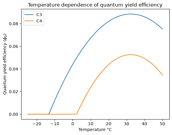
The default approach (method_kphio='temperature', QuantumYieldTemperature) applies a temperature dependent estimate of \(\phi_0\), following Bernacchi et al. (2003) for C3 plants and Cai and Prentice (2020) for C4 plants.

Show code cell source

Hide code cell source

# Calculate temperature dependence of quantum yield efficiency
env = PModelEnvironment(tc=tc_1d, patm=101325, vpd=820, co2=40, fapar=1, ppfd=1)

fkphio_c3 = QuantumYieldTemperature(env=env, use_c4=False)
fkphio_c4 = QuantumYieldTemperature(env=env, use_c4=True)

# Create a line plot of ftemp kphio
plt.plot(tc_1d, fkphio_c3.kphio, label="C3")
plt.plot(tc_1d, fkphio_c4.kphio, label="C4")

plt.title("Temperature dependence of quantum yield efficiency")
plt.xlabel("Temperature °C")
plt.ylabel(r"Quantum yield efficiency ($\phi_0$)")
plt.legend()
plt.show()

Fixed \(\phi_0\)

This approach (method_kphio='fixed', QuantumYieldFixed) applies a fixed value of \(\phi_0\) in the calculation of light use efficiency.

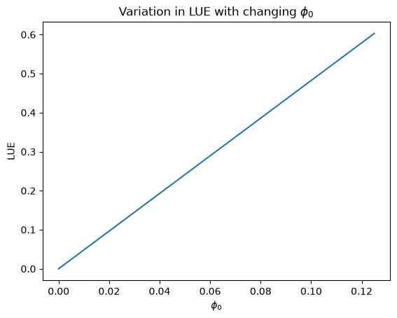
However, the fixed method will also accept \(\phi_0\) values for each observation being fitted in the PModel. This option is provided to allow users to experiment with alternative per-observation estimation of \(\phi_0\) that are not currently implemented. You will need to provide an array of values that has the same shape as the other driver variables and these values are then used within the calculations for each observation.

In the code and plot below, this approach is used to provide a simple linear series of \(\phi_0\) values to an otherwise constant environment. As you would expect given \(\text{LUE} = \phi_0 \cdot M_C \cdot m_j\), light use efficiency changes linearly along this gradient of \(\phi_0\) values.

Show code cell source

Hide code cell source

# A constant environment to show a range of kphio values
kphio_values = np.arange(0, 0.126, step=0.001)
n_vals = len(kphio_values)

env = PModelEnvironment(
    tc=np.repeat(20, n_vals),
    patm=np.repeat(101325, n_vals),
    vpd=np.repeat(820, n_vals),
    co2=np.repeat(400, n_vals),
    fapar=np.repeat(1, n_vals),
    ppfd=np.repeat(1, n_vals),
)
model_var_kphio = PModel(env, method_kphio="fixed", reference_kphio=kphio_values)

# Create a line plot of ftemp kphio
plt.plot(kphio_values, model_var_kphio.lue)
plt.title(r"Variation in LUE with changing $\phi_0$")
plt.xlabel(r"$\phi_0$")
plt.ylabel("LUE")
plt.show()

/home/docs/checkouts/readthedocs.org/user_builds/pyrealm/checkouts/latest/pyrealm/pmodel/pmodel.py:481: UserWarning: 
            The default value for quantum yield of photosynthesis (phi0=1/8) has changed
            since pyrealm 1.0.0. You may need to change settings to duplicate results 
            from pyrealm 1.0.0.
            
  warn(

Temperature and aridity effects on \(\phi_0\)

Warning

This approach is parameterised from data and uses a fixed estimate of maximum \(\phi_0 \approx 1/9\). You cannot alter the maximum value using the reference_kphio argument.

Sandoval et al. (2026) implemented a new method (method_kphio='sandoval', QuantumYieldSandoval), where \(\phi_0\) is calculated as a function of a local aridity index (calculated as PET / P), the mean growth temperature and the air temperature (Sandoval et al., 2026). You will need to provide the aridity index and mean growing temperature for observations when creating the PModelEnvironment.

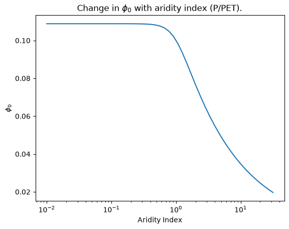
First, the aridity index is used to adjust the reference value (\(\phi_{0R}\)) using a double exponential function to calculate a new maximum value given the climatological aridity (\(\phi_{0A}\)):

\[ \phi_{0A} = \dfrac{\phi_{0R}}{(1 + \textrm{AI}^m) ^ n} \]

This captures a decrease in maximum \(\phi_0\) in arid conditions, as shown below.

Show code cell source

Hide code cell source

n_vals = 51
aridity_index = np.logspace(-2, 1.5, num=n_vals)

env = PModelEnvironment(
    tc=np.repeat(20, n_vals),
    patm=np.repeat(101325, n_vals),
    vpd=np.repeat(820, n_vals),
    co2=np.repeat(400, n_vals),
    fapar=np.repeat(1, n_vals),
    ppfd=np.repeat(1, n_vals),
    aridity_index=aridity_index,
    mean_growth_temperature=np.repeat(20, n_vals),
)

sandoval_kphio = QuantumYieldSandoval(env)

fig, ax = plt.subplots(1, 1)
ax.plot(aridity_index, sandoval_kphio.kphio)
ax.set_title(r"Change in $\phi_0$ with aridity index (P/PET).")
ax.set_ylabel(r"$\phi_0$")
ax.set_xlabel("Aridity Index")
ax.set_xscale("log")
plt.show()

/home/docs/checkouts/readthedocs.org/user_builds/pyrealm/checkouts/latest/pyrealm/core/experimental.py:72: ExperimentalFeatureWarning: 'Be aware that QuantumYieldSandoval is an experimental feature of pyrealm and the implementation and API may change within major versions.'
  warn(qualname, ExperimentalFeatureWarning)

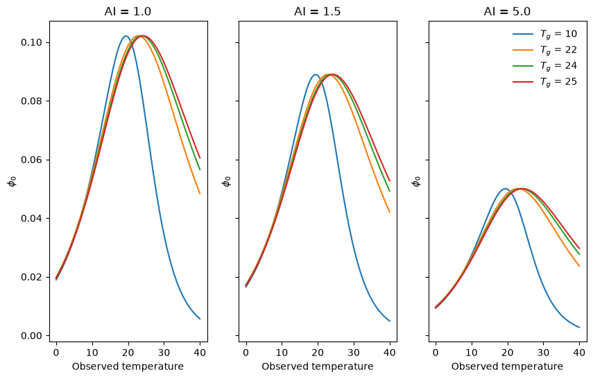
In addition to capping the peak \(\phi_0\) as a function of the aridity index, the method also captures how plants adjust peak efficiency to their conditions. A peaked Arrhenius model is used to calculate the realised \(\phi_0\) given both the current temperature and the mean growth temperature (\(T_g\)) for observations. The plot below shows how aridity and mean growth temperature interact to change the location and height of the peak \(\phi_0\) and how realised \(\phi_0\) at a temperature varies given the mean growth temperature.

Show code cell source

Hide code cell source

n_vals = 51
mean_growth_values = np.array([10, 22, 24, 25])
aridity_values = np.array([1.0, 1.5, 5.0])
tc_values = np.linspace(0, 40, n_vals)

shape = (n_vals, len(aridity_values), len(mean_growth_values))

ai3, tc3, mg3 = np.meshgrid(aridity_values, tc_values, mean_growth_values)


env = PModelEnvironment(
    tc=tc3,
    patm=np.full(shape, 101325),
    vpd=np.full(shape, 820),
    co2=np.full(shape, 400),
    fapar=np.full(shape, 1),
    ppfd=np.full(shape, 1),
    aridity_index=ai3,
    mean_growth_temperature=mg3,
)

sandoval_kphio = QuantumYieldSandoval(env)

fig, axes = plt.subplots(ncols=3, nrows=1, sharey=True, figsize=(10, 6))

for ai_idx, (ax, ai_val) in enumerate(zip(axes, aridity_values)):

    for mg_idx, mg_val in enumerate(mean_growth_values):
        ax.plot(
            env.tc[:, ai_idx, mg_idx],
            sandoval_kphio.kphio[:, ai_idx, mg_idx],
            label=f"$T_{{g}}$ = {mg_val}",
        )
        ax.set_title(f"AI = {ai_val}")
        ax.set_ylabel(r"$\phi_0$")
        ax.set_xlabel("Observed temperature")


ax.legend(frameon=False)
plt.show()