Allometry in the T Model

Run this notebook

• Read the guide on setting up your computer to run Jupyter notebooks

• Download this notebook as a Jupyter notebook.

import warnings

from matplotlib import pyplot as plt
import numpy as np
import pandas as pd

from pyrealm.core.experimental import ExperimentalFeatureWarning
from pyrealm.demography.flora import Flora
from pyrealm.demography.cohorts import create_cohorts, cohort_id_generator
from pyrealm.demography.tmodel import StemAllometry

warnings.filterwarnings(
    "ignore",
    category=ExperimentalFeatureWarning,
)

To generate allometric predictions under the T Model, we need to define a set of cohorts:

# Create a flora with 3 PFTs with different maximum heights
flora = Flora(name=["short", "medium", "tall"], h_max=[10, 20, 30])

# Create an id generator.
cid_generator = cohort_id_generator(mode="str")

# Create the cohorts
cohorts = create_cohorts(
    flora=flora,
    cid_generator=cid_generator,
    pft_name=np.array(["short", "medium", "tall"]),
    dbh_value=np.array([0.1, 0.1, 0.1]),
    n_individuals=np.array([1, 1, 1]),
)

Stem allometry

We can visualise how the stem size, canopy size and various masses of PFTs change with stem diameter by using the StemAllometry class. Creating a StemAllometry instance needs an existing Flora instance and an array of values for diameter at breast height (DBH, metres). The returned class contains the predictions of the T Model for:

• Stem height (stem_height, m),

• Crown area (crown_area, m2),

• Crown fraction (crown_fraction, -),

• Stem mass (stem_mass, kg),

• Foliage mass (foliage_mass, kg),

• Sapwood mass (sapwood_mass, kg),

• Crown radius scaling factor (crown_r0, -), and

• Height of maximum crown radius (crown_z_max, m).

Note that stem_height denotes the total tree height, as used interchangeable in Li et al. (2014), rather than just the height of the trunk below the canopy.

The DBH input can be a scalar array or a one dimensional array providing a single value for each PFT. This then calculates a single estimate at the given size for each stem.

# Calculate the allometry for the cohorts
cohort_allometry = StemAllometry(cohorts=cohorts)
cohort_allometry

StemAllometry: Allometry predictions for 3 cohorts.

The StemAllometry() class provides the to_dataframe() method to export the stem data for data exploration. The StemAllometry data retains the unique cohort ids and DBH from the original cohort data.

cohort_allometry.to_dataframe().transpose()

	0	1	2
cohort_ids	C_000000	C_000001	C_000002
dbh	0.1	0.1	0.1
stem_height	6.865138	8.802033	9.620475
crown_area	1.814782	2.326795	2.543148
crown_fraction	0.591822	0.758796	0.829351
stem_mass	5.391867	6.9131	7.555903
foliage_mass	0.233329	0.299159	0.326976
fine_root_mass	0.555323	0.711999	0.778203
sapwood_mass	4.493533	6.5109	7.335868
crown_r0	0.261731	0.296362	0.309834
crown_z_max	5.83731	7.484219	8.180126

Allometry profiles

The at_dbh argument to StemAllometry can be used to generate profiles of the allometry predictions for PFTs at different sizes. The provided values are used to calculate predictions instead of the cohort DBH values. The allometry attributes of predictions are then 2 dimensional arraus arranged with each cohort as a column and each DBH prediction as a row. This makes them convenient to plot using matplotlib.

# Column array of DBH values from 0.01 to 1.6 metres
dbh_profile = np.arange(0.01, 1.6, 0.01)
# Get the predictions at those DBH values.
allometry_profiles = StemAllometry(cohorts=cohorts, at_dbh=dbh_profile)

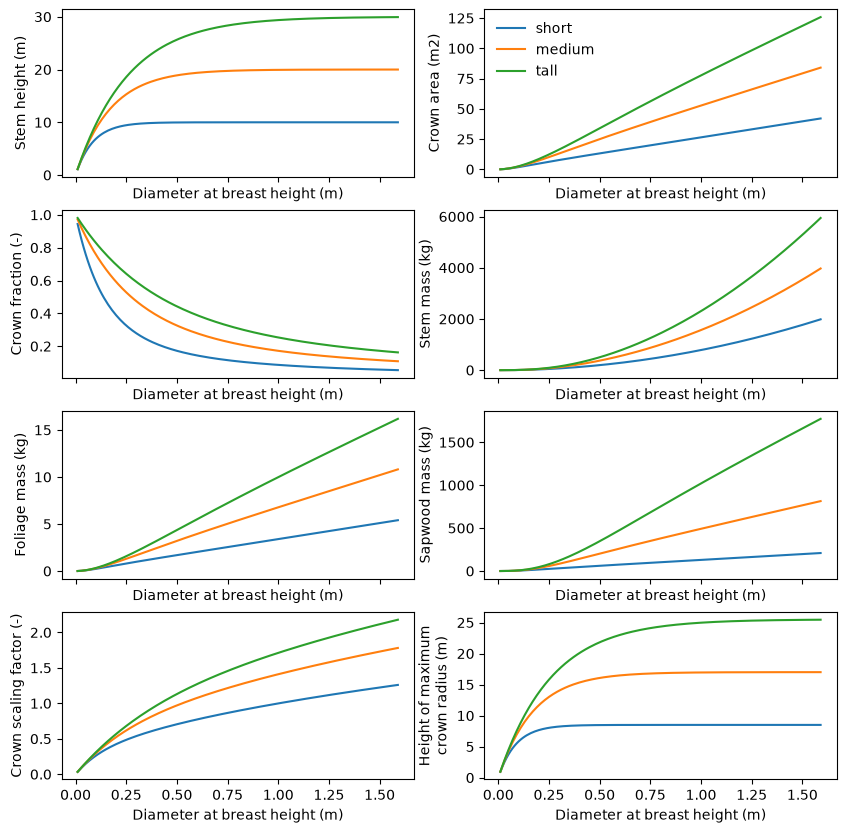
The code below shows how to use the returned allometries to generate a plot of the scaling relationships across all of the PFTs in a Flora instance.

fig, axes = plt.subplots(ncols=2, nrows=4, sharex=True, figsize=(10, 10))

plot_details = [
    ("stem_height", "Stem height (m)"),
    ("crown_area", "Crown area (m2)"),
    ("crown_fraction", "Crown fraction (-)"),
    ("stem_mass", "Stem mass (kg)"),
    ("foliage_mass", "Foliage mass (kg)"),
    ("sapwood_mass", "Sapwood mass (kg)"),
    ("crown_r0", "Crown scaling factor (-)"),
    ("crown_z_max", "Height of maximum\ncrown radius (m)"),
]

for ax, (var, ylab) in zip(axes.flatten(), plot_details):
    ax.plot(dbh_profile, getattr(allometry_profiles, var), label=flora.name)
    ax.set_xlabel("Diameter at breast height (m)")
    ax.set_ylabel(ylab)

    if var == "crown_area":
        ax.legend(frameon=False)

The to_dataframe() method can still be used, but the values are stacked into columns identified by pairings of cohort ID and DBH.

allometry_profiles.to_dataframe().head(6)[
    ["cohort_ids", "dbh", "stem_height", "crown_area", "crown_fraction"]
]

	cohort_ids	dbh	stem_height	crown_area	crown_fraction
0	C_000000	0.01	1.095248	0.028953	0.944179
1	C_000001	0.01	1.127001	0.029792	0.971553
2	C_000002	0.01	1.137860	0.030079	0.980913
3	C_000000	0.02	2.070539	0.109468	0.892474
4	C_000001	0.02	2.190496	0.115810	0.944179
5	C_000002	0.02	2.232562	0.118034	0.962311