Soil moisture effects

Run this notebook

• Read the guide on setting up your computer to run Jupyter notebooks

• Download this notebook as a Jupyter notebook.

Approaches to modelling the impact of soil moisture conditions on photosynthesis are a very open area and a number of different methods are implemented in pyrealm. These different approaches reflect uncertainty about the most appropriate way to modulate predictions.

Warning

The soil moisture approaches described on this page should not be combined with each other. In addition, some of these methods were calibrated for a particular form of the P Model or with particular settings and so should be used with models that follow those particular settings.

Alternative approaches

Effects on optimal chi

The pyrealm package includes two separate approaches that affect optimal chi:

• The lavergne20_c3 (OptimalChiLavergne20C3) and lavergne20_c4 (OptimalChiLavergne20C4) methods , which use an empirical model of the change in the ratio of the photosynthetic costs of carboxilation and transpiration.

• The experimental optimal chi methods that impose a direct rootzone stress penalty on the \(\beta\) term in calculating optimal chi: prentice14_rootzonestress (OptimalChiPrentice14RootzoneStress), c4_rootzonestress (OptimalChiC4RootzoneStress), and c4_no_gamma_rootzonestress (OptimalChiC4NoGammaRootzoneStress)

Effects on the quantum yield of photosynthesis

• The sandoval method (QuantumYieldSandoval) implements an experimental calculation that modulates \(\phi_0\) as a function of the temperature and a local aridity index.

Post-hoc penalties on gross primary productivity

These approaches both use empirical functions of soil moisture and aridity data that have been parameterised to align raw predictions from a P Model with field observations of GPP. Two penalty function are available that calculate the fraction of potential GPP that is realised given the effects of soil moisture stress:

• The calculate_soilmstress_stocker() function implements the Stocker et al. (2020) GPP penalty for use with the standard P Model.

• calculate_soilmstress_mengoli() function implements the Mengoli et al. (2023) GPP penalty for use with the subdaily P Model.

The GPP penalty functions are described in more detail below, using the artificial data set created below. The data set consists of 5 days of observations of a constant environment that can be used to show the effects of changing soil moisture input values on the resulting GPP.

Show code cell source

Hide code cell source

from matplotlib import pyplot as plt
import numpy as np

from pyrealm.pmodel import (
    PModelEnvironment,
    PModel,
    calculate_soilmstress_stocker,
    calculate_soilmstress_mengoli,
    SubdailyPModel,
    AcclimationModel,
)
from pyrealm.constants import PModelConst

# Create a test data set consisting of 5 days of observations of a constant environment
# that can be used to show the effects of changing soil moisture input values on the
# resulting GPP
n_obs = 48 * 5
obs_minutes = 30
time_offsets = np.arange(0, n_obs * obs_minutes, obs_minutes).astype("timedelta64[m]")
datetimes = np.datetime64("2000-01-01 00:00") + time_offsets

# Constant P Model environment
env = PModelEnvironment(
    tc=np.full(n_obs, fill_value=20),
    patm=np.full(n_obs, fill_value=101325),
    vpd=np.full(n_obs, fill_value=820),
    co2=np.full(n_obs, fill_value=400),
    fapar=np.full(n_obs, fill_value=1),
    ppfd=np.full(n_obs, fill_value=1000),
)

# Soil moisture gradient across the observations
sm_gradient = np.linspace(0, 1.0, n_obs)

The calculate_soilmstress_stocker() penalty factor

This calculates an empirically derived penalty factor based on soil moisture (\(\theta\)) (Stocker et al., 2020, Stocker et al., 2018) that captures the loss of gross primary productivity (GPP) resulting from soil moisture stress.

The factor \(\beta(\theta) \in [0,1]\) requires estimates of:

• relative soil moisture (\(m_s\), soilm), as the fraction of field capacity, and

• a measure of local mean aridity (\(\bar{\alpha}\), meanalpha), as the average annual ratio of AET to PET.

Soil moisture

The parameters used in the calculation of this factor were estimated using the plant-available soil water expressed as a fraction of available water holding capacity. That capacity was calculated for the observed data on a site by site basis using the SoilGrids dataset (Hengl et al., 2017). Ideally, soil moisture calculated in the same way should be used with this approach.

The functions to calculate \(\beta(\theta)\) are based on four parameters, derived from experimental data and set in PModelConst:

• An upper bound in relative soil moisture (\(\theta^\ast\), soilmstress_thetastar), above which \(\beta\) is always 1, corresponding to no loss of light use efficiency.

• An lower bound in relative soil moisture (\(\theta_0\), soilmstress_theta0), below which LUE is always zero.

• An intercept (a, soilmstress_a) for the aridity sensitivity parameter \(q\).

• A slope (b, soilmstress_b) for the aridity sensitivity parameter \(q\).

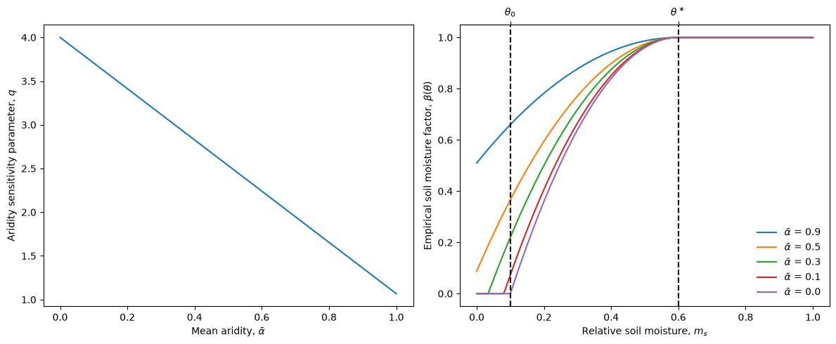
The aridity measure (\(\bar{\alpha}\)) is first used to set an aridity sensitivity parameter (\(q\)), which sets the speed with which \(\beta(\theta) \to 0\) as \(m_s\) decreases.

\[ q = \frac{(1 - (a + b \bar{\alpha}))}{(\theta^\ast - \theta_{0})^2} \]

Then, relative soil moisture (\(m_s\)) is used to calculate the soil moisture factor:

\[ \beta(\theta) = q ( m_s - \theta^\ast) ^ 2 + 1 \]

The figures below shows how the aridity sensitivity parameter (\(q\)) changes with differing aridity measures and then how the soil moisture factor \(\beta(\theta)\) varies with changing soil moisture for differing values of mean aridity. In the examples below, the default \(\theta_0 = 0\) has been changed to \(\theta_0 = 0.1\) to make the lower bound more obvious.

Show code cell source

Hide code cell source

# change default theta0 parameter
coef = PModelConst().soilmstress_stocker
coef["theta0"] = 0.1

# Calculate q
mean_alpha_seq = np.linspace(0, 1, n_obs)

q = (1 - (coef["a"] + coef["b"] * mean_alpha_seq)) / (
    coef["thetastar"] - coef["theta0"]
) ** 2

# Create a 1x2 plot
fig, (ax1, ax2) = plt.subplots(1, 2, figsize=(12, 5))

# Plot q ~ mean_alpha
ax1.plot(mean_alpha_seq, q)
ax1.set_xlabel(r"Mean aridity, $\bar{\alpha}$")
ax1.set_ylabel(r"Aridity sensitivity parameter, $q$")


for mean_alpha in [0.9, 0.5, 0.3, 0.1, 0.0]:

    soilmstress = calculate_soilmstress_stocker(
        soilm=sm_gradient, meanalpha=mean_alpha, coef=coef
    )
    ax2.plot(
        sm_gradient, soilmstress, label=r"$\bar{{\alpha}}$ = {}".format(mean_alpha)
    )

ax2.axvline(x=coef["thetastar"], linestyle="--", color="black")
ax2.axvline(x=coef["theta0"], linestyle="--", color="black")

secax = ax2.secondary_xaxis("top")
secax.set_xticks(
    ticks=[coef["thetastar"], coef["theta0"]],
    labels=[r"$\theta^\ast$", r"$\theta_0$"],
)

ax2.legend(frameon=False)
ax2.set_xlabel(r"Relative soil moisture, $m_s$")
ax2.set_ylabel(r"Empirical soil moisture factor, $\beta(\theta)$")

plt.tight_layout()

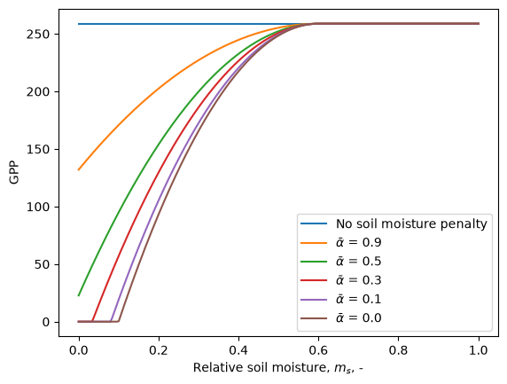
Application of the calculate_soilmstress_stocker() factor

The factor can be applied to the P Model by using calculate_soilmstress_stocker() to calculate the factor values and then multiplying calculated GPP (gpp) by the resulting factor. The example below shows how the predicted light use efficiency from the P Model changes across an aridity gradient both with and without the soil moisture factor.

In the rpmodel implementation, the soil moisture factor is applied within the calculation of the P Model and the penalised GPP is used to modify \(V_{cmax}\) and \(J_{max}\), so that these values are congruent with the resulting penalised LUE and GPP. This is not implemented in the pmodel module, where correction is only implemented as a post-hoc penalty to GPP.

Caution

• This soil moisture stress function was parameterised using the standard P Model (PModel) and is unlikely to transfer well to GPP predictions from the subdaily form of the model (SubdailyPModel).

• The parameterisation of this soil moisture stress function formed part of a wider model tuning in Stocker et al. (2020) that also adjusted the value of the quantum yield of photosynthesis to capture canopy scale efficiency. To match this calibration process, the correction should be applied to outputs of a PModel with matching settings: see calculate_soilmstress_stocker() for details.

# Configure the PModel to use the 'BRC' model setup of Stocker et al. (2020)
model = PModel(
    env=env,
    method_kphio="temperature",
    method_arrhenius="simple",
    method_jmaxlim="wang17",
    method_optchi="prentice14",
    reference_kphio=0.081785,
)

# Calculate the soil moisture stress factor across a soil moisture gradient
# at differing aridities

gpp_stressed = {}

for mean_alpha in [0.9, 0.5, 0.3, 0.1, 0.0]:
    # Calculate the stress for this aridity
    sm_stress = calculate_soilmstress_stocker(
        soilm=sm_gradient, meanalpha=mean_alpha, coef=coef
    )
    # Apply the penalty factor
    gpp_stressed[mean_alpha] = model.gpp * sm_stress

/home/docs/checkouts/readthedocs.org/user_builds/pyrealm/checkouts/latest/pyrealm/pmodel/pmodel.py:481: UserWarning: 
    Pyrealm 2.0.0 uses a new default for the quantum yield of photosynthesis (phi0=1/8).
    You may need to change settings to duplicate results from pyrealm 1.0.0.
            
  warn(

Show code cell source

Hide code cell source

plt.plot(sm_gradient, model.gpp, label="No soil moisture penalty")

for ky, val in gpp_stressed.items():
    plt.plot(sm_gradient, val, label=r"$\bar{{\alpha}}$ = {}".format(ky))

plt.xlabel(r"Relative soil moisture, $m_s$, -")
plt.ylabel(r"GPP")
plt.legend()
plt.show()

The calculate_soilmstress_mengoli() penalty factor

This is an empirically derived factor (\(\beta(\theta) \in [0,1]\), (Mengoli et al., 2023) that describes a penalty to gross primary productivity (GPP) resulting from soil moisture stress.

The factor requires estimates of:

• relative soil moisture (\(m_s\), soilm), as the fraction of field capacity, and

• a climatological estimate of local aridity index, typically calculated as total PET over total precipitation for an appropriate period, typically at least 20 years.

Soil moisture

The parameters used in the calculation of this factor were estimated using the plant-available soil water expressed as the ratio of millimeters of soil moisture over the total soil capacity. The soil water estimated using CRU data in SPLASH v1 model (Davis et al., 2017), which enforces a constant soil capacity of 150mm. Again, ideally, soil moisture calculated in the same way should be used with this approach.

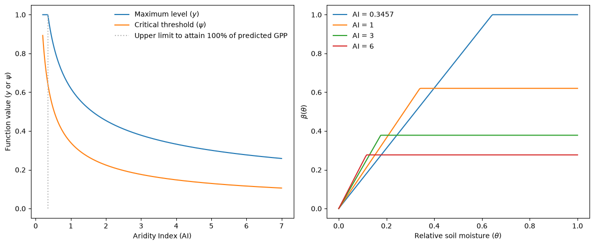
The calculation of \(\beta(\theta)\) is based on two functions of the aridity index. Both functions are power laws, constrained to take a maximum of 1 (no soil moisture stress penalty). The first function describes the maximal attainable level (\(y\)) and the second function describes a threshold (\(\psi\)) at which that level is reached. The parameters of these power laws are derived from experimental data and set in PModelConst.

\[\begin{split} \begin{align*} y &= \min( a \textrm{AI} ^ {b}, 1)\\ \psi &= \min( a \textrm{AI} ^ {b}, 1)\\ \end{align*} \end{split}\]

The penalty factor \(\beta(\theta)\) is then calculated given the relative soil moisture \(\theta\), the threshold \(\psi\) and the maximum level:

\[\begin{split} \beta(\theta) = \begin{cases} y, & \theta \ge \psi \\ \dfrac{y}{\psi} \cdot \theta, & \theta \lt \psi \end{cases} \end{split}\]

The function for the maximum attainable level \(y\) reaches the maximum value of 1 at:

\[ \textrm{AI} = e^{-log(a)/b} \]

Given the default values, this critical level is around 0.3457: plants can only realise the predicted GPP from the P Model in locations where the aridity index is less than this value.

coef = PModelConst().soilmstress_mengoli
print(coef)

{'psi_a': 0.34, 'psi_b': -0.6, 'y_a': 0.62, 'y_b': -0.45}

AI_crit_y = np.exp(-np.log(coef["y_a"]) / coef["y_b"])
round(AI_crit_y, 4)

np.float64(0.3457)

aridity_index = np.sort(np.concatenate([[AI_crit_y], np.linspace(0.2, 7, n_obs)]))

y = np.minimum(coef["y_a"] * np.power(aridity_index, coef["y_b"]), 1)

psi = np.minimum(
    coef["psi_a"] * np.power(aridity_index, coef["psi_b"]),
    1,
)

# Create a 1x2 plot
fig, (ax1, ax2) = plt.subplots(1, 2, figsize=(12, 5))

ax1.plot(aridity_index, y, label="Maximum level ($y$)")
ax1.plot(aridity_index, psi, label="Critical threshold ($\psi$)")
ax1.plot(
    [AI_crit_y, AI_crit_y],
    [0, 1],
    linestyle=":",
    color="0.7",
    label="Upper limit to attain 100% of predicted GPP",
)
ax1.set_xlabel(r"Aridity Index (AI)")
ax1.set_ylabel(r"Function value ($y$ or $\psi$)")
ax1.legend(frameon=False)


# Calculate the soil moisture stress factor across a soil moisture
# gradient for different aridity index values
beta = {}
ai_vals = [AI_crit_y.round(4), 1, 3, 6]

for ai in ai_vals:
    beta[ai] = calculate_soilmstress_mengoli(
        soilm=sm_gradient, aridity_index=np.array(ai)
    )
    plt.plot(sm_gradient, beta[ai], label=f"AI = {ai}")

ax2.set_xlabel(r"Relative soil moisture ($\theta$)")
ax2.set_ylabel(r"$\beta(\theta)$")
ax2.legend(frameon=False)

plt.tight_layout()

<>:14: SyntaxWarning: invalid escape sequence '\p'
<>:14: SyntaxWarning: invalid escape sequence '\p'
/tmp/ipykernel_1539/3662894310.py:14: SyntaxWarning: invalid escape sequence '\p'
  ax1.plot(aridity_index, psi, label="Critical threshold ($\psi$)")

np.exp(-np.log(0.62) / -0.45)

np.float64(0.3456592624095148)

As the plots above show, plants in arid conditions have severely constrained maximum levels, but have lower critical thresholds, allowing them to maintain the maximum level under drier conditions.

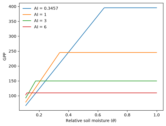
Application of the calculate_soilmstress_mengoli() factor

As with calculate_soilmstress_stocker(), the factor is first calculated and then applied to the GPP calculated for a model (gpp). In the example below, the result is obviously just \(\beta(\theta)\) from above scaled to the constant GPP.

Caution

• This soil moisture stress function was parameterised using the subdaily P Model (SubdailyPModel) and is unlikely to transfer well to GPP predictions from the standard form of the model (PModel).

• The parameterisation of this soil moisture stress function was estimated using predictions from a particular parameterisation of the subdaily PModel. To match the parameterisation settings, the correction should be applied to outputs of a SubdailyPModel with matching settings: see calculate_soilmstress_mengoli() for details.

acclim_model = AcclimationModel(datetimes=datetimes)
acclim_model.set_window(
    window_center=np.timedelta64(12, "h"), half_width=np.timedelta64(1, "h")
)

subdaily_model = SubdailyPModel(
    env=env,
    acclim_model=acclim_model,
    method_kphio="temperature",
    method_arrhenius="simple",
    method_jmaxlim="wang17",
    method_optchi="prentice14",
    reference_kphio=1 / 8,
)

for ai in ai_vals:

    plt.plot(sm_gradient, subdaily_model.gpp * beta[ai], label=f"AI = {ai}")

plt.xlabel(r"Relative soil moisture ($\theta$)")
plt.ylabel("GPP")
plt.legend(frameon=False)
plt.show()