Using the Two Leaf, Two Stream model

Run this notebook

• Read the guide on setting up your computer to run Jupyter notebooks

• Download this notebook as a Jupyter notebook.

from importlib import resources

import xarray
import numpy as np
import matplotlib.pyplot as plt
from matplotlib.colors import Normalize
import matplotlib.cm as cm
import matplotlib.dates as mdates

from pyrealm.core.solar import SolarPositions
from pyrealm.pmodel.pmodel import PModel, SubdailyPModel
from pyrealm.pmodel.pmodel_environment import PModelEnvironment
from pyrealm.pmodel.acclimation import AcclimationModel
from pyrealm.pmodel.two_leaf import TwoLeafIrradiance, TwoLeafAssimilation

from pyrealm.core.hygro import convert_sh_to_vpd

This page shows how to use the two leaf, two stream model of assimilation (De Pury and Farquhar, 1997) in pyrealm. The standard and subdaily P Model use the big leaf approximation of the canopy structure: assimilation is estimated as if all the available light falls directly as a beam onto a single large leaf. In the two leaf, two stream model, De Pury and Farquhar (1997) differentiate the absorbance of light into sunlit and shaded leaves (‘two leaf’) and also into direct and scattered radiation (‘two streams’). Within the canopy, the model separates out beam, scattered and diffuse irradiation and estimates how much of each stream is absorbed by the sunlit and shaded leaves.

The example code below uses the same dataset as the subdaily worked example, which is a two month extract of WFDE5 data for the United Kingdom:

• time: 2018-06-01 00:00 to 2018-07-31 23:00 at 1 hour resolution.

• longitude: 10°W to 4°E at 0.5° resolution.

• latitude: 49°N to 60°N at 0.5° resolution

The code uses a subset of this wider arrays data to three sites to plot time series.

# Loading the example dataset:
dpath = (
    resources.files("pyrealm_build_data.uk_data") / "UK_WFDE5_FAPAR_2018_JuneJuly.nc"
)
ds = xarray.load_dataset(dpath)

datetimes = ds["time"]

# Define three sites for showing time series
sites = xarray.Dataset(
    data_vars=dict(
        lat=(["stid"], [50.73, 53.93, 58.03]), lon=(["stid"], [-3.52, -0.79, -4.41])
    ),
    coords=dict(stid=(["Exeter", "Pocklington", "Lairg"])),
)

The WFDE data need some conversion for use in the PModel, along with the definition of the atmospheric CO2 concentration.

# Variable set up
# Air temperature in °C from Tair in Kelvin
tc = ds["Tair"] - 273.15
# Atmospheric pressure in Pascals
patm = ds["PSurf"]
# Convert specific humidity to VPD and remove negative values
vpd = convert_sh_to_vpd(sh=ds["Qair"], ta=tc, patm=patm / 1000) * 1000
vpd = np.clip(vpd, 0, np.inf)
# Extract fAPAR (unitless)
fapar = ds["fAPAR"]
# Convert SW downwelling radiation from W/m^2 to PPFD µmole/m2/s1
ppfd = ds["SWdown"] * 2.04
# Define atmospheric CO2 concentration (ppm)
co2 = np.ones_like(tc) * 400

Fitting big leaf models

In pyrealm, we use an initial big leaf model (either a standard or subdaily P Model) to estimate four parameters that are required for the two leaf, two stream model. These are:

• The maximum rates of carboxylation at the observation and standard temperatures (\(V_{cmax}\) and \(V_{cmax25}\)).

• The limitation terms on rates of carboxylation (\(m_c\)) and electron transfer (\(m_j\)) from the calculation of optimal chi.

So the first step in calculating two leaf, two stream estimates is to fit a P Model:

# Generate and check the PModelEnvironment
pm_env = PModelEnvironment(tc=tc, patm=patm, vpd=vpd, co2=co2, fapar=fapar, ppfd=ppfd)

# Fit a standard P Model
standard_bigleaf = PModel(
    env=pm_env,
    method_kphio="fixed",
    method_optchi="prentice14",
)

# Create an acclimation model to fit a subdaily model
acclim_model = AcclimationModel(datetimes, alpha=1 / 15, allow_holdover=True)
acclim_model.set_window(
    window_center=np.timedelta64(12, "h"),
    half_width=np.timedelta64(1, "h"),
)

# Fit a Subdaily P Model
subdaily_bigleaf = SubdailyPModel(
    env=pm_env,
    acclim_model=acclim_model,
    method_optchi="prentice14",
    method_kphio="fixed",
)

/home/docs/checkouts/readthedocs.org/user_builds/pyrealm/checkouts/latest/pyrealm/pmodel/pmodel.py:481: UserWarning: 
    Pyrealm 2.0.0 uses a new default for the quantum yield of photosynthesis (phi0=1/8).
    You may need to change settings to duplicate results from pyrealm 1.0.0.
            
  warn(

Estimating solar elevation and irradiances

In contrast to the big leaf model, where light hits a single flat surface, the two leaf, two stream model models a canopy with depth and where the behaviour of light varies with the angle of solar elevation. Lower angles lead to more light scattering, because of the longer light path through the atmosphere, and then light penetration into the canopy varies with incident angle.

The SolarPositions class can be used to calculate solar elevation for observations, given the latitude, longitude and time of an observation. The code below takes the latitude, longitude and time coordinates of the example data and converts them into three dimensional arrays, so that the solar elevations of all observations can be calculated.

# Convert latitude, longitude and time coordinates into 3D arrays
datetime_array, latitude_array, longitude_array = np.meshgrid(
    datetimes, ds.lat, ds.lon, indexing="ij"
)

# Calculate solar positions
solar_pos = SolarPositions(
    latitude=latitude_array,
    longitude=longitude_array,
    datetime=datetime_array,
)

The SolarPositions object contains more detailed solar data (such as the hour angle), but the critical parameter for the two leaf, two stream model is the solar elevation.

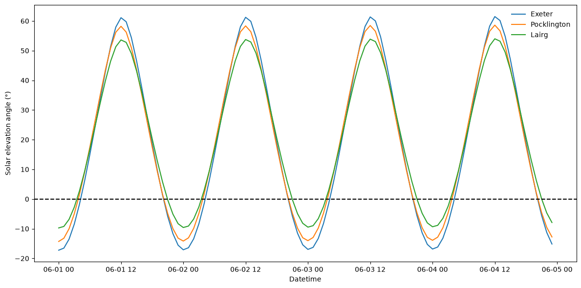
The plot below shows the resulting solar elevation curves for three sites from the gridded data. The elevations show the expected patterns for the summer in the Northern Hemisphere: more northly sites have lower consistently elevation angles but also have shorter night times (solar elevation < 0°).

# Store the predictions in the xarray Dataset to use indexing
ds["solar_elevation"] = (ds["Tair"].dims, solar_pos.solar_elevation)

# Get a four day time series of the three sites
site_ds = ds.sel(sites, method="nearest")
site_ds = site_ds.where(site_ds.time < np.datetime64("2018-06-05"), drop=False)

# Plot solar elevation for each site
fig, ax = plt.subplots(figsize=(12, 6))
for st in sites["stid"].values:

    ax.plot(
        site_ds["time"],
        np.rad2deg(site_ds["solar_elevation"].sel(stid=st)),
        label=st,
    )

ax.axhline(0, linestyle="--", color="k")
ax.set_xlabel("Datetime")
ax.set_ylabel("Solar elevation angle (°)")
plt.legend(frameon=False)
plt.tight_layout()

These solar elevation values can then be used to calculate the irradiances absorbed by sunlit and shaded leaves within the two-leaf, two-stream models. These values are independent of the type of P Model being used, so the calculations can be used across multiple P Models. The irradiance calculation requires:

• the solar elevation (\(\beta\)) in radians,

• the photosynthetic photon flux density (PPFD) in µmol m-2 s-1,

• the leaf area index (\(L\)) of the canopy, and

• the atmospheric pressure.

irradiances = TwoLeafIrradiance(
    solar_elevation=solar_pos.solar_elevation,
    ppfd=ppfd,
    leaf_area_index=2,
    patm=patm,
)

/home/docs/checkouts/readthedocs.org/user_builds/pyrealm/checkouts/latest/pyrealm/core/experimental.py:72: ExperimentalFeatureWarning: 'Be aware that TwoLeafIrradiance is an experimental feature of pyrealm and the implementation and API may change within major versions.'
  warn(qualname, ExperimentalFeatureWarning)
/home/docs/checkouts/readthedocs.org/user_builds/pyrealm/checkouts/latest/pyrealm/pmodel/two_leaf.py:328: RuntimeWarning: overflow encountered in power
  f_d = (1 - atmos_transmission_par**m) / (
/home/docs/checkouts/readthedocs.org/user_builds/pyrealm/checkouts/latest/pyrealm/pmodel/two_leaf.py:329: RuntimeWarning: overflow encountered in power
  1 + (atmos_transmission_par**m * (1 / atmospheric_scattering - 1))
/home/docs/checkouts/readthedocs.org/user_builds/pyrealm/checkouts/latest/pyrealm/pmodel/two_leaf.py:328: RuntimeWarning: invalid value encountered in divide
  f_d = (1 - atmos_transmission_par**m) / (
/home/docs/checkouts/readthedocs.org/user_builds/pyrealm/checkouts/latest/pyrealm/pmodel/two_leaf.py:337: UserWarning: Negative diffuse radiation fractions clamped to zero.
  warn("Negative diffuse radiation fractions clamped to zero.")

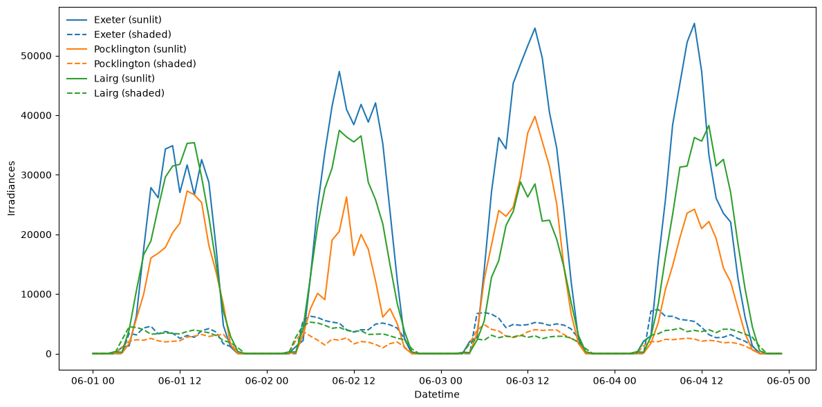
The plot below shows the resulting absorbed radiation for the two leaf types for the three sites.

Caution

The shortwave downwelling radiation used here is a “ground level” estimate accounting for cloud cover, which is why the plots show a jagged profile. This may not be appropriate for use with the two leaf, two stream model.

# Store the predictions in the xarray Dataset to use indexing
ds["sunlit_absorbed_irradiance"] = (
    ds["Tair"].dims,
    irradiances.sunlit_absorbed_irradiance,
)
ds["shaded_absorbed_irradiance"] = (
    ds["Tair"].dims,
    irradiances.shaded_absorbed_irradiance,
)


# Get a four day time series of the three sites
site_ds = ds.sel(sites, method="nearest")
site_ds = site_ds.where(site_ds.time < np.datetime64("2018-06-05"), drop=False)

# Plot solar elevation for each site
fig, ax = plt.subplots(figsize=(12, 6))
for st, col in zip(sites["stid"].values, ("C0", "C1", "C2")):

    ax.plot(
        site_ds["time"],
        np.rad2deg(site_ds["sunlit_absorbed_irradiance"].sel(stid=st)),
        label=st + " (sunlit)",
        color=col,
    )

    ax.plot(
        site_ds["time"],
        np.rad2deg(site_ds["shaded_absorbed_irradiance"].sel(stid=st)),
        label=st + " (shaded)",
        linestyle="--",
        color=col,
    )

ax.set_xlabel("Datetime")
ax.set_ylabel("Irradiances")
plt.legend(frameon=False)
plt.tight_layout()

Assimilation under the two leaf, two stream model

The last step is to calculate the assimilation resulting from those irradiance values, given the estimated photosynthetic behaviour from the P Model, using the TwoLeafAssimilation class. A detailed description of the calculations are given in the API documentation for the class, but in brief:

• The carboxylation capacity (\(V_cmax\)) varies with depth in the canopy, where we use leaf area index (\(L\)) to represent canopy depth (Lloyd et al., 2010).

• The resulting standardized carboxylation capacity \(V_{cmax25}\) through the canopy is partitioned between sunlit and shaded leaves.

• Currently, the standardized electron transfer capacity \(J_{max25}\) is calculated as an empirical function of \(V_{cmax25}\) for sunlit and shaded leaves (Wullschleger, 1993).

• The Arrhenius scaling method used with the P Model is then used to adjust these estimates at standard temperature to the actual temperature. estimates to the observed temperatures.

• Separately for sunlit and shaded leaves, the limitation terms from the calculation of optimal \(\chi\) are then used to calculate the actual maximum assimilation via the carboxylation (\(A_v\)) and electron transfer (\(A_j\)) pathways and then the realised assimilation (\(A = \min \left( A_{v}, A_{j} \right)\)).

• The sum of the realised sunlit and shaded assimilation then gives the total assimilation, which is multiplied by the molar mass of carbon to express GPP as µg C m-2 s-1.

# Calculate the two leaf assimilation
standard_two_leaf = TwoLeafAssimilation(pmodel=standard_bigleaf, irradiance=irradiances)
subdaily_two_leaf = TwoLeafAssimilation(pmodel=subdaily_bigleaf, irradiance=irradiances)

/home/docs/checkouts/readthedocs.org/user_builds/pyrealm/checkouts/latest/pyrealm/core/experimental.py:72: ExperimentalFeatureWarning: 'Be aware that TwoLeafAssimilation is an experimental feature of pyrealm and the implementation and API may change within major versions.'
  warn(qualname, ExperimentalFeatureWarning)

# Store the predictions in the xarray Dataset to use indexing
ds["standard_big_leaf"] = (ds["Tair"].dims, standard_bigleaf.gpp)
ds["subdaily_big_leaf"] = (ds["Tair"].dims, subdaily_bigleaf.gpp)
ds["standard_two_leaf"] = (ds["Tair"].dims, standard_two_leaf.gpp)
ds["subdaily_two_leaf"] = (ds["Tair"].dims, subdaily_two_leaf.gpp)

# Get a four day time series of the three sites
site_ds = ds.sel(sites, method="nearest")
site_ds = site_ds.where(site_ds.time < np.datetime64("2018-06-05"), drop=False)

# Plot solar elevation for each site
fig, axes = plt.subplots(nrows=3, ncols=2, figsize=(10, 8), sharex=True, sharey=True)

for (lax, rax), st in zip(axes, sites["stid"].values):

    lax.plot(
        site_ds["time"],
        site_ds["standard_big_leaf"].sel(stid=st),
    )
    lax.plot(
        site_ds["time"],
        site_ds["standard_two_leaf"].sel(stid=st),
    )

    rax.plot(
        site_ds["time"],
        site_ds["subdaily_big_leaf"].sel(stid=st),
        label="Big leaf",
    )

    rax.plot(
        site_ds["time"],
        site_ds["subdaily_two_leaf"].sel(stid=st),
        label="Two leaf",
    )

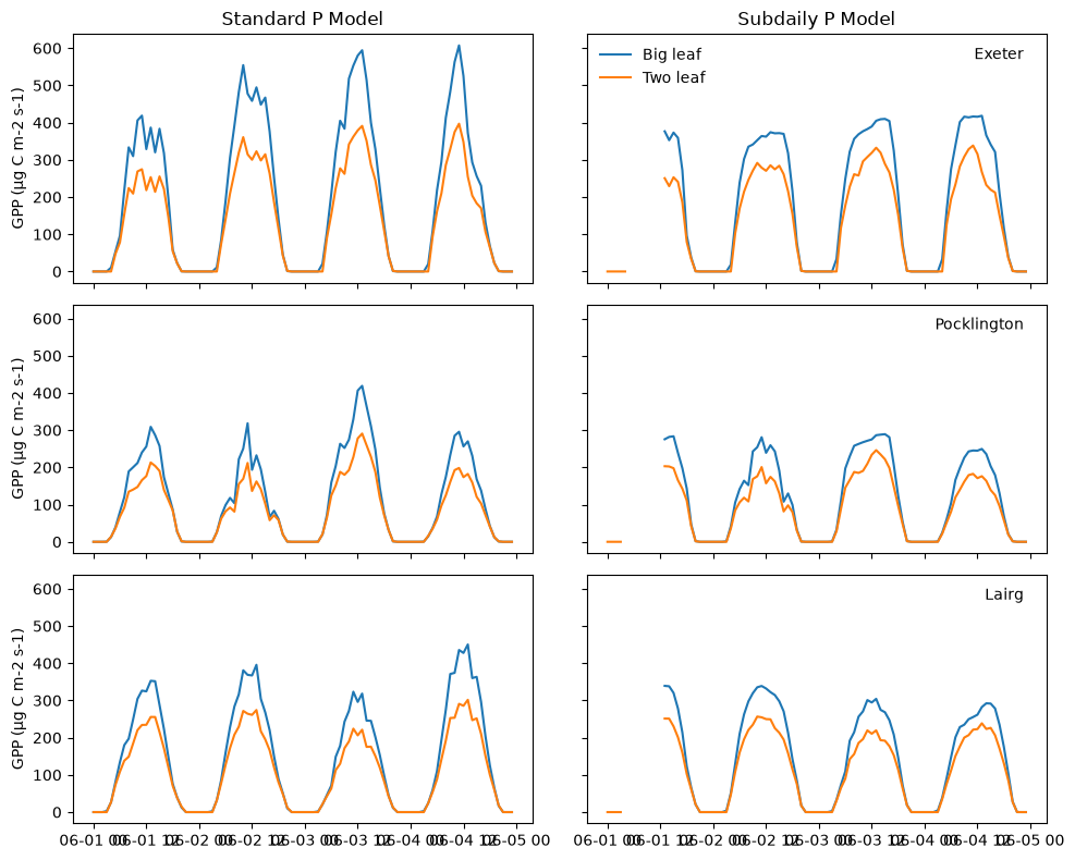
    # Annotations
    lax.set_ylabel("GPP (µg C m-2 s-1)")
    rax.text(0.95, 0.9, st, ha="right", transform=rax.transAxes)
    if st == "Exeter":
        lax.set_title("Standard P Model")
        rax.set_title("Subdaily P Model")
        rax.legend(frameon=False)


plt.tight_layout()

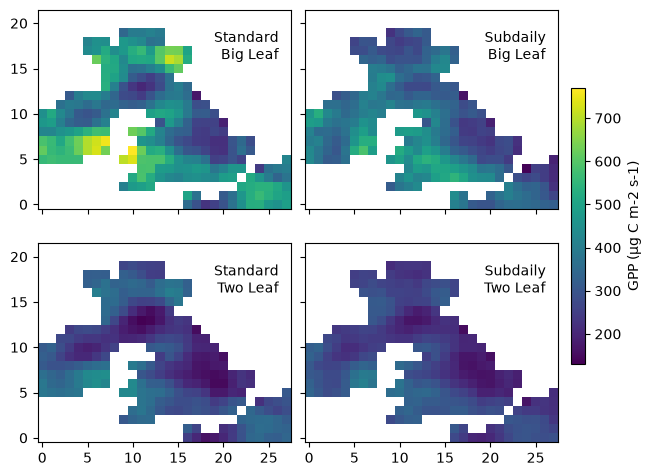
The plots above have extracted site-specific time series to show temporal patterns, but the calculations of GPP have been conducted across the whole of the spatial grid. The plot below shows the comparative estimates of GPP from the four model fitted for a noon observation.

single_time = ds.where(ds.time == np.datetime64("2018-06-04 12:00:00"), drop=True)

# Shared image scale
gpp_data = np.concatenate(
    [
        single_time["standard_big_leaf"],
        single_time["subdaily_big_leaf"],
        single_time["standard_two_leaf"],
        single_time["subdaily_two_leaf"],
    ]
)
gpp_min = np.nanmin(gpp_data)
gpp_max = np.nanmax(gpp_data)


fig, axes = plt.subplots(
    ncols=2, nrows=2, layout="constrained", sharex=True, sharey=True
)

ax1, ax2, ax3, ax4 = axes.flatten()
cm = ax1.imshow(
    single_time["standard_big_leaf"].squeeze(),
    vmin=gpp_min,
    vmax=gpp_max,
    origin="lower",
)
ax2.imshow(
    single_time["subdaily_big_leaf"].squeeze(),
    vmin=gpp_min,
    vmax=gpp_max,
    origin="lower",
)
ax3.imshow(
    single_time["standard_two_leaf"].squeeze(),
    vmin=gpp_min,
    vmax=gpp_max,
    origin="lower",
)
ax4.imshow(
    single_time["subdaily_two_leaf"].squeeze(),
    vmin=gpp_min,
    vmax=gpp_max,
    origin="lower",
)

labels = (
    "Standard\nBig Leaf",
    "Subdaily\nBig Leaf",
    "Standard\nTwo Leaf",
    "Subdaily\nTwo Leaf",
)

for ax, lab in zip(axes.flatten(), labels):
    ax.text(0.95, 0.9, lab, va="top", ha="right", transform=ax.transAxes)


_ = plt.colorbar(
    cm, ax=axes[:, 1], location="right", shrink=0.6, label="GPP (µg C m-2 s-1)"
)