Worked examples
This page shows two worked examples of how to use pyrealm to make predictions using
the P Model.
Run this notebook
Read the guide on setting up your computer to run Jupyter notebooks
Download
this notebookas a Jupyter notebook.
The first example uses a single point but the second shows how the package can be used
with array data. The pyrealm package uses the numpy package and expects inputs to
be passed either as single scalar values, or as arrays with shapes that are consistent
under broadcasting rules. See the page on array inputs for
details.
from importlib import resources

from matplotlib import pyplot as plt
import numpy as np
import xarray

from pyrealm.pmodel.pmodel import PModel
from pyrealm.pmodel import PModelEnvironment
from pyrealm.core.pressure import calculate_patm
Warning
The pyrealm package uses a modular approach to define many of the shared
components of the standard and subdaily P Model.
Some combinations of the methods implemented may modify the same aspect of the model
using different approaches.
As an example, there are multiple approaches to incorporating effects of soil moisture stress on productivity, via modulation of \(\phi_0\), \(m_j\) and the calculation of GPP penalty factors.
At present, pyrealm does not automatically check the compatibility of method
selection, so take care when setting methods options for fitting a P Model.
Simple point estimate
This example calculates a single point estimate of GPP. The first step is to use
estimates of environmental variables to calculate the
photosynthetic environment for the model
(PModelEnvironment).
The example shows the steps required using a single site with:
a temperature of 20°C,
standard atmospheric at sea level (101325 Pa),
a vapour pressure deficit of 0.82 kPa (~ 65% relative humidity), and
an atmospheric \(\ce{CO2}\) concentration of 400 ppm.
Estimating productivity
The PModelEnvironment also accepts estimates
of the fraction of absorbed photosynthetically active radiation (\(f_{APAR}\), fapar,
unitless) and the photosynthetic photon flux density (PPFD,ppfd, µmol m-2 s-1).
Together these are used to calculate the absorbed irradiance, which is used to scale up
the estimated light use efficiency to estimate the actual productivity of the model.
Here we are using:
An absorption fraction of 0.91 (-), and
a PPFD of 834 µmol m-2 s-1.
Warning
In the PModelEnvironment(), the estimated PPFD
must be expressed as µmol m-2 s-1.
Estimates of PPFD sometimes use different temporal or spatial scales - for example daily moles of photons per hectare. Although GPP can also be expressed with different units, many other predictions of the P Model (\(J_{max}\), \(V_{cmax}\), \(g_s\) and \(r_d\)) must be expressed as µmol m-2 s-1 and so this standard unit must also be used for PPFD.
# Calculate the PModelEnvironment
env = PModelEnvironment(tc=20.0, patm=101325.0, vpd=820, co2=400, fapar=0.91, ppfd=834)
env
PModelEnvironment(shape=(1,))
The env object now holds the photosynthetic environment, which can be reused with
different P Model settings. The representation of a
PModelEnvironment object (env) is
deliberately terse - just the shape of the data - but the
PModelEnvironment.summarize
method provides a more detailed summary of the attributes.
env.summarize()
PModelEnvironment(shape=(1,))
Attr            Mean        Min        Max    NaN  Units
---------  ---------  ---------  ---------  -----  ------------
tc             20         20         20         0  °C
vpd           820        820        820         0  Pa
co2           400        400        400         0  ppm
patm       101325     101325     101325         0  Pa
fapar           0.91       0.91       0.91      0  -
ppfd          834        834        834         0  µmol m-2 s-1
ca             40.53      40.53      40.53      0  Pa
gammastar       3.34       3.34       3.34      0  Pa
kmm            46.1       46.1       46.1       0  Pa
ns_star         1.13       1.13       1.13      0  -
Fitting the P Model
Next, the P Model can be fitted to the photosynthetic environment using the
(PModel) class:
model = PModel(env)
/home/docs/checkouts/readthedocs.org/user_builds/pyrealm/checkouts/latest/pyrealm/pmodel/pmodel.py:481: UserWarning:
            The default value for quantum yield of photosynthesis (phi0=1/8) has changed
            since pyrealm 1.0.0. You may need to change settings to duplicate results
            from pyrealm 1.0.0.

  warn(
The returned model object holds a lot of information. The representation of the model object shows a terse display of the settings used to run the model:
model
PModel(shape=(1,), method_optchi=prentice14, method_arrhenius=simple, method_jmaxlim=wang17, method_kphio=temperature)
A PModel instance also has a
summarize() method that summarizes settings and
displays a summary of calculated predictions. Initially, this shows two measures of
photosynthetic efficiency: the intrinsic water use efficiency (iwue) and the light
use efficiency (lue).
model.summarize()
PModel(shape=(1,), method_optchi=prentice14, method_arrhenius=simple, method_jmaxlim=wang17, method_kphio=temperature)
Attr       Mean     Min     Max    NaN  Units
-------  ------  ------  ------  -----  ------------
lue        0.4     0.4     0.4       0  g C mol-1
iwue      71.45   71.45   71.45      0  µmol mol-1
gpp      300.21  300.21  300.21      0  µg C m-2 s-1
vcmax     73.25   73.25   73.25      0  µmol m-2 s-1
vcmax25  114.82  114.82  114.82      0  µmol m-2 s-1
gs         2.16    2.16    2.16      0  µmol m-2 s-1
jmax     167.72  167.72  167.72      0  µmol m-2 s-1
jmax25   226.86  226.86  226.86      0  µmol m-2 s-1
\(\chi\) estimates and \(\ce{CO2}\) limitation
The instance also contains a OptimalChiPrentice14
object,
recording key parameters from the calculation of
\(\chi\).
This object also has a summarize()
method:
model.optchi.summarize()
OptimalChiPrentice14(shape=(1,))
Attr      Mean    Min    Max    NaN  Units
------  ------  -----  -----  -----  ----------
xi       63.3   63.3   63.3       0  Pa ^ (1/2)
chi       0.71   0.71   0.71      0  -
mc        0.34   0.34   0.34      0  -
mj        0.72   0.72   0.72      0  -
mjoc      2.11   2.11   2.11      0  -
3D grid example
This example shows how the pmodel module can be used with array inputs
to calculate a global map of gross primary productivity (GPP).
First, we load some
example data from a NetCDF format file using the excellent xarray package.
These data are 0.5° global grids containing data for 2 months and so the loaded
data are three dimensional arrays and shape (2, 360, 720) .
# Load an example dataset containing the forcing variables.
data_path = resources.files("pyrealm_build_data.rpmodel") / "pmodel_global.nc"
ds = xarray.load_dataset(data_path)

# Extract the six variables for the two months
temp = ds["temp"]
co2 = ds["CO2"]
elev = ds["elevation"]
vpd = ds["VPD"]
fapar = ds["fAPAR"]
ppfd = ds["ppfd"]
The model can now be run using that data. The first step is to convert the elevation data to atmospheric pressure, and then this is used to set the photosynthetic environment for the model:
# Convert elevation to atmospheric pressure
patm = calculate_patm(elev)

# Mask out temperature values below -25°C
temp = temp.where(temp >= -25)

# Clip VPD to force negative VPD to be zero
vpd = np.clip(vpd, 0, np.inf)

# Calculate the photosynthetic environment
env = PModelEnvironment(tc=temp, co2=co2, patm=patm, vpd=vpd, fapar=fapar, ppfd=ppfd)
env.summarize()
PModelEnvironment(shape=(2, 360, 720))
Attr           Mean       Min        Max     NaN  Units
---------  --------  --------  ---------  ------  ------------
tc             4.11    -25         33.6   387580  °C
vpd         1119.03      2.76    5379.87  332622  Pa
co2          390.68    390.2      391.17       0  ppm
patm       97367.9   50317.1   102175          0  Pa
fapar          0.32      0          0.99  414897  -
ppfd       38690.1       0     254494          0  µmol m-2 s-1
ca            38.04     19.63      39.97       0  Pa
gammastar      2.04      0.12       6.53  387580  Pa
kmm           31.46      0.62     147.5   387580  Pa
ns_star        2.28      0.83       5.62  387580  -
/home/docs/checkouts/readthedocs.org/user_builds/pyrealm/checkouts/latest/pyrealm/core/bounds.py:173: UserWarning: Variable 'ppfd' (µmol m-2 s-1) contains values outside the expected range (0,3000). Check units?
  warn(
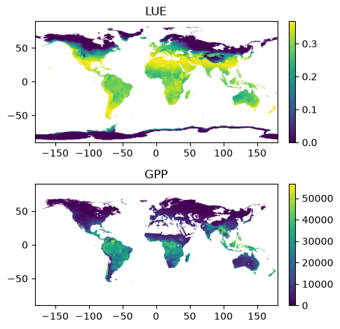
That environment can then be run to calculate the P model predictions for GPP:
# Run the P model
model = PModel(env)

fig, (ax1, ax2) = plt.subplots(2, 1)

# Plot LUE for first month
im = ax1.imshow(model.lue[0, :, :], origin="lower", extent=[-180, 180, -90, 90])
plt.colorbar(im, fraction=0.022, pad=0.03, ax=ax1)
ax1.set_title("LUE")

im = ax2.imshow(model.gpp[0, :, :], origin="lower", extent=[-180, 180, -90, 90])
plt.colorbar(im, fraction=0.022, pad=0.03, ax=ax2)
ax2.set_title("GPP")

plt.tight_layout()
/home/docs/checkouts/readthedocs.org/user_builds/pyrealm/checkouts/latest/pyrealm/pmodel/pmodel.py:481: UserWarning:
            The default value for quantum yield of photosynthesis (phi0=1/8) has changed
            since pyrealm 1.0.0. You may need to change settings to duplicate results
            from pyrealm 1.0.0.

  warn(