Worked example of the Subdaily P Model

Run this notebook

• Read the guide on setting up your computer to run Jupyter notebooks

• Download this notebook as a Jupyter notebook.

from importlib import resources

import xarray
import numpy as np
import matplotlib.pyplot as plt
from matplotlib.colors import Normalize
import matplotlib.cm as cm
import matplotlib.dates as mdates

from pyrealm.pmodel.pmodel import PModel, SubdailyPModel
from pyrealm.pmodel.pmodel_environment import PModelEnvironment
from pyrealm.pmodel.acclimation import AcclimationModel

from pyrealm.core.hygro import convert_sh_to_vpd

This notebook shows example analyses fitting P Models that include fast and slow photosynthetic responses to subdaily variation in environmental conditions. The dataset is taken from WFDE5 v2 and provides 1 hourly resolution data on a 0.5° spatial grid. The fAPAR data is interpolated to the same spatial and temporal resolution from MODIS data.

• time: 2018-06-01 00:00 to 2018-07-31 23:00 at 1 hour resolution.

• longitude: 10°W to 4°E at 0.5° resolution.

• latitude: 49°N to 60°N at 0.5° resolution

This notebook demonstrates fitting subdaily P Models in the pyrealm package. Model fitting basically takes all of the same arguments as the standard PModel class. There are three additional things to set:

• The timing of the observations and the daily window that should be used to estimate acclimation of slow responses.

• How rapidly plants acclimate to daily optimal conditions.

• Approaches to handling any missing data: since estimating acclimation involves a recursive function, the subdaily model can be derailed by missing or undefined data.

The test data use some UK WFDE data for three sites in order to compare predictions over a time series.

# Loading the example dataset:
dpath = (
    resources.files("pyrealm_build_data.uk_data") / "UK_WFDE5_FAPAR_2018_JuneJuly.nc"
)
ds = xarray.load_dataset(dpath)

datetimes = ds["time"]

# Define three sites for showing time series
sites = xarray.Dataset(
    data_vars=dict(
        lat=(["stid"], [50.73, 53.93, 58.03]), lon=(["stid"], [-3.52, -0.79, -4.41])
    ),
    coords=dict(stid=(["Exeter", "Pocklington", "Lairg"])),
)

The WFDE data need some conversion for use in the PModel, along with the definition of the atmospheric CO2 concentration.

# Variable set up
# Air temperature in °C from Tair in Kelvin
tc = ds["Tair"] - 273.15
# Atmospheric pressure in Pascals
patm = ds["PSurf"]
# Convert specific huidity to VPD and remove negative values
vpd = convert_sh_to_vpd(sh=ds["Qair"], ta=tc, patm=patm / 1000) * 1000
vpd = np.clip(vpd, 0, np.inf)
# Extract fAPAR (unitless)
fapar = ds["fAPAR"]
# Convert SW downwelling radiation from W/m^2 to PPFD µmole/m2/s1
ppfd = ds["SWdown"] * 2.04
# Define atmospheric CO2 concentration (ppm)
co2 = np.ones_like(tc) * 400

The code below then calculates the photosynthetic environment.

# Generate and check the PModelEnvironment
pm_env = PModelEnvironment(tc=tc, patm=patm, vpd=vpd, co2=co2, fapar=fapar, ppfd=ppfd)
pm_env.summarize()

PModelEnvironment(shape=(1464, 22, 28))
Attr            Mean       Min        Max     NaN  Units
---------  ---------  --------  ---------  ------  ------------
tc             16.18      2.11      36.96  499224  °C
vpd           524.12      0       5017.47  499224  Pa
co2           400       400        400          0  ppm
patm       100240     92628.5   103125     499224  Pa
fapar           0.57      0          0.83  439200  -
ppfd          470.53      0       1883.22  499224  µmol m-2 s-1
ca             40.1      37.05      41.25  499224  Pa
gammastar       2.77      1.16       7.65  499224  Pa
kmm            35.9       9.82     196.7   499224  Pa
ns_star         1.25      0.78       1.86  499224  -

Instantaneous C3 and C4 P Models

The standard implementation of the P Model used below assumes that plants can instantaneously adopt optimal behaviour.

# Standard PModels
pmodC3 = PModel(
    env=pm_env,
    method_kphio="fixed",
    method_optchi="prentice14",
)
pmodC3.summarize()

PModel(shape=(1464, 22, 28), method_optchi=prentice14, method_arrhenius=simple, method_jmaxlim=wang17, method_kphio=fixed)
Attr       Mean    Min     Max     NaN  Units
-------  ------  -----  ------  ------  ------------
lue        0.67   0.25    0.87  499224  g C mol-1
iwue      62.54  -0      93.77  499224  µmol mol-1
gpp      174.57   0     925.51  499224  µg C m-2 s-1
vcmax     40.39   0     260.12  499224  µmol m-2 s-1
vcmax25   73.42   0     471.73  499224  µmol m-2 s-1
gs         1.36   0     189.84  500224  µmol m-2 s-1
jmax      96.07   0     498.7   499224  µmol m-2 s-1
jmax25   148.77   0     975.21  499224  µmol m-2 s-1

/home/docs/checkouts/readthedocs.org/user_builds/pyrealm/checkouts/latest/pyrealm/pmodel/pmodel.py:481: UserWarning: 
    Pyrealm 2.0.0 uses a new default for the quantum yield of photosynthesis (phi0=1/8).
    You may need to change settings to duplicate results from pyrealm 1.0.0.
            
  warn(

pmodC4 = PModel(
    env=pm_env,
    method_kphio="fixed",
    method_optchi="c4_no_gamma",
)

pmodC4.summarize()

PModel(shape=(1464, 22, 28), method_optchi=c4_no_gamma, method_arrhenius=simple, method_jmaxlim=wang17, method_kphio=fixed)
Attr       Mean    Min      Max     NaN  Units
-------  ------  -----  -------  ------  ------------
lue        1.01   1.01     1.01       0  g C mol-1
iwue     131.8    0      169.27  499224  µmol mol-1
gpp      282.42   0     1515.53  499224  µg C m-2 s-1
vcmax     85.72   0      866.79  499224  µmol m-2 s-1
vcmax25  146.08   0      874.39  499224  µmol m-2 s-1
gs         1.04   0       71.32  500224  µmol m-2 s-1
jmax     126.61   0      679.4   499224  µmol m-2 s-1
jmax25   192.23   0     1176.13  499224  µmol m-2 s-1

np.nanmean(pmodC3.iwue)

np.float64(62.53942906917798)

np.nanmean((pmodC3.gpp / pmodC3.env.core_const.k_c_molmass) / pmodC3.gs)

/tmp/ipykernel_1654/2943314788.py:1: RuntimeWarning: invalid value encountered in divide
  np.nanmean((pmodC3.gpp / pmodC3.env.core_const.k_c_molmass) / pmodC3.gs)

np.float64(10.386864418595097)

Subdaily P Models

The code below then refits these models, with slow responses in \(\xi\), \(V_{cmax25}\) and \(J_{max25}\). The allow_holdover argument allows the estimation of realised optimal values to holdover previous realised values to cover missing data within the calculations: essentially the plant does not acclimate until the optimal values can be calculated again to update those realised estimates.

# Set the acclimation window to an hour either side of noon
acclim_model = AcclimationModel(datetimes, alpha=1 / 15, allow_holdover=True)
acclim_model.set_window(
    window_center=np.timedelta64(12, "h"),
    half_width=np.timedelta64(1, "h"),
)

# Fit C3 and C4 with the Subdaily P Model
subdailyC3 = SubdailyPModel(
    env=pm_env,
    acclim_model=acclim_model,
    method_optchi="prentice14",
    method_kphio="fixed",
)
subdailyC4 = SubdailyPModel(
    env=pm_env,
    acclim_model=acclim_model,
    method_optchi="c4_no_gamma",
    method_kphio="fixed",
)

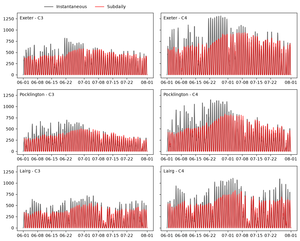
Time series predictions

The code below then extracts the time series for the two months from the three sites shown above and plots the instantaneous predictions against predictions including slow photosynthetic responses.

# Store the predictions in the xarray Dataset to use indexing
ds["GPP_pmodC3"] = (ds["Tair"].dims, pmodC3.gpp)
ds["GPP_subdailyC3"] = (ds["Tair"].dims, subdailyC3.gpp)
ds["GPP_pmodC4"] = (ds["Tair"].dims, pmodC4.gpp)
ds["GPP_subdailyC4"] = (ds["Tair"].dims, subdailyC4.gpp)

# Get three sites to show time series for locations
site_ds = ds.sel(sites, method="nearest")

# Set up subplots
fig, axes = plt.subplots(3, 2, figsize=(10, 8), sharey=True)

# Plot the time series for the two approaches for each site
for (ax1, ax2), st in zip(axes, sites["stid"].values):

    ax1.plot(
        datetimes,
        site_ds["GPP_pmodC3"].sel(stid=st),
        label="Instantaneous",
        color="0.4",
    )
    ax1.plot(
        datetimes,
        site_ds["GPP_subdailyC3"].sel(stid=st),
        label="Subdaily",
        color="red",
        alpha=0.7,
    )
    ax1.xaxis.set_major_formatter(mdates.DateFormatter("%m-%d"))
    ax1.text(0.02, 0.90, st + " - C3", transform=ax1.transAxes)

    ax2.plot(
        datetimes,
        site_ds["GPP_pmodC4"].sel(stid=st),
        label="Instantaneous",
        color="0.4",
    )
    ax2.plot(
        datetimes,
        site_ds["GPP_subdailyC4"].sel(stid=st),
        label="Subdaily",
        color="red",
        alpha=0.7,
    )
    ax2.xaxis.set_major_formatter(mdates.DateFormatter("%m-%d"))
    ax2.text(0.02, 0.90, st + " - C4", transform=ax2.transAxes)

axes[0][0].legend(loc="lower center", bbox_to_anchor=[0.5, 1], ncols=2, frameon=False)
plt.tight_layout()

Converting models

The subdaily models can also be obtained directly from the standard models, using the PModel.to_subdaily method:

# Convert standard C3 model
converted_C3 = pmodC3.to_subdaily(acclim_model=acclim_model)

# Convert standard C4 model
converted_C4 = pmodC4.to_subdaily(acclim_model=acclim_model)

This produces the same outputs as the SubdailyPModel class, but is convenient and more compact when the two models are going to be compared.