The tree crown model

Run this notebook

• Read the guide on setting up your computer to run Jupyter notebooks

• Download this notebook as a Jupyter notebook.

Warning

This area of pyrealm is in active development and this notebook currently contains notes and initial demonstration code.

from matplotlib import pyplot as plt
from matplotlib.lines import Line2D
from matplotlib.patches import Polygon, Patch
import numpy as np
import pandas as pd

from pyrealm.demography.flora import (
    calculate_crown_q_m,
    calculate_crown_z_max_proportion,
    PlantFunctionalType,
    Flora,
)

from pyrealm.demography.tmodel import (
    calculate_dbh_from_height,
    StemAllometry,
)

from pyrealm.demography.crown import (
    CrownProfile,
    get_crown_xy,
)

The pyrealm.demography module uses three-dimensional model of crown shape to define the vertical distribution of leaf area, following the implementation of crown shape in the Plant-FATE model (Joshi et al., 2022).

Crown traits

The crown model for a plant functional type (PFT) is driven by four traits within the PlantFunctionalType class:

• The m and n (\(m, n\)) traits set the vertical shape of the crown profile.

• The ca_ratio trait sets the area of the crown (\(A_c\)) relative to the stem size.

• The f_g (\(f_g\)) trait sets the crown gap fraction and sets the vertical distribution of leaves within the crown.

Canopy shape

For a stem of height \(H\), the \(m\) and \(n\) traits are used to calculate the relative crown radius \(q(z)\) at a height \(z\) of as:

\[ q(z)= m n \left(\dfrac{z}{H}\right) ^ {n -1} \left( 1 - \left(\dfrac{z}{H}\right) ^ n \right)^{m-1} \]

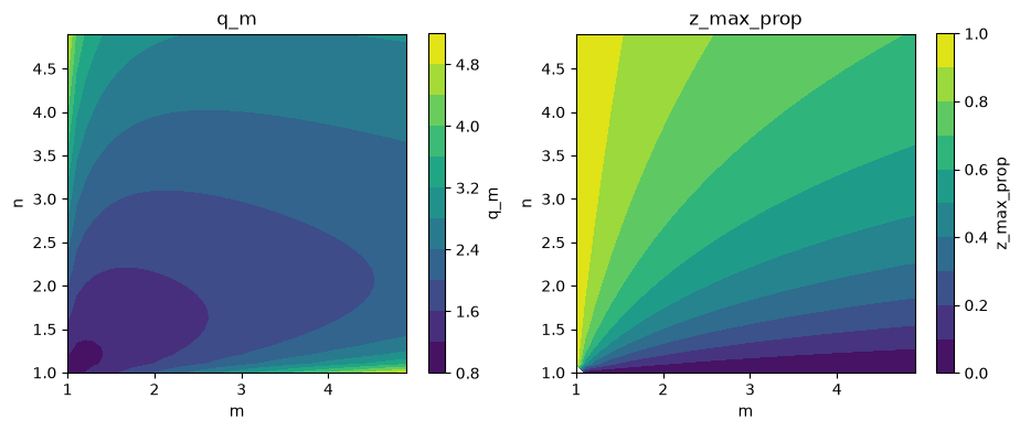
In order to align the arbitrary relative radius values with the predictions of the T Model for the stem, we then need to find the height at which the relative radius is at its maximum and a scaling factor that will convert the relative area at this height to the expected crown area under the T Model. These can be calculated using the following two additional traits, which are invariant for a PFT.

• z_max_prop (\(p_{zm}\)) sets the proportion of the height of the stem at which the maximum relative crown radius is found.

• q_m (\(q_m\)) is used to scale the size of the crown radius at \(z_{max}\) to match the expected crown area.

\[\begin{split} \begin{align} p_{zm} &= \left(\dfrac{n-1}{m n -1}\right)^ {\tfrac{1}{n}}\\[8pt] q_m &= m n \left(\dfrac{n-1}{m n -1}\right)^ {1 - \tfrac{1}{n}} \left(\dfrac{\left(m-1\right) n}{m n -1}\right)^ {m-1} \end{align} \end{split}\]

For individual stems, with expected height \(H\) and crown area \(A_c\), we can then calculate:

• the height \(z_m\) at which the maximum crown radius \(r_m\) is found,

• a height-specific scaling factor \(r_0\) such that \(\pi q(z_m)^2 = A_c\),

• the actual crown radius \(r(z)\) at a given height \(z\).

\[\begin{split} \begin{align} z_m &= H p_{zm}\\[8pt] r_0 &= \frac{1}{q_m}\sqrt{\frac{A_c}{\pi}}\\[8pt] r(z) &= r_0 \; q(z) \end{align} \end{split}\]

Projected crown and leaf area

From the crown radius profile, the model can then be used to calculate how crown area and leaf area accumulates from the top of the crown towards the ground, giving functions given height \(z\) for:

• the projected crown area \(A_p(z)\), and

• the projected leaf area \(\tilde{A}_{cp}(z)\).

The projected crown area is calculated for a stem of known height and crown area is:

\[\begin{split} A_p(z)= \begin{cases} A_c, & z \le z_m \\ A_c \left(\dfrac{q(z)}{q_m}\right)^2, & H > z > z_m \\ 0, & z > H \end{cases} \end{split}\]

That is, the projected crown area is zero above the top of the stem, increases to the expected crown area at \(z_max\) and is then constant to ground level.

The projected leaf area \(\tilde{A}_{cp}(z)\) models how the vertical distribution of leaf area within the crown is modified by the crown gap fraction (\(f_g\)). This trait captures the relative canopy openness of different plant functional types. Some PFTs occupy a large space in the canopy but have relatively open crowns that let light pass down into canopy more. Other PFTs form compact crowns that are arranged a more closed surface.

If we compare two PFTs that only differ in \(f_g\), then they will have exactly the same projected crown areas at a given height, and this drives how the tree takes up space within the canopy. However the PFT with the larger \(f_g\) will have a more open canopy, with leaf area over a wider vertical range within the canopy shape because of the increased openness of the canopy. When \(f_g = 0\), the projected crown and leaf areas are identical, but as \(f_g \to 1\) the projected leaf area is pushed downwards.

Put another way, a stem has a total leaf surface area defined by the crown area and the characteristic leaf area index of the plant functional type. The crown gap fraction effectively tunes where vertically in the crown shape of the tree that LAI is deployed: when \(f_g = 0\) the leaf area is concentrated exactly at the upper surface of the crown but, as \(f_g \to 1\), more and more of leaf surface is deployed more deeply through the broader shape of the tree crown. Crown gaps do not extend all the way to the ground, just to other parts of the crown further down in the crown.

The calculation of \(\tilde{A}_{cp}(z)\) is defined as:

\[\begin{split} \tilde{A}_{cp}(z)= \begin{cases} 0, & z \gt H \\ A_c \left(\dfrac{q(z)}{q_m}\right)^2 \left(1 - f_g\right), & H \gt z \gt z_m \\ Ac - A_c \left(\dfrac{q(z)}{q_m}\right)^2 f_g, & zm \gt z \end{cases} \end{split}\]

Calculating crown model traits in pyrealm

The PlantFunctionalType class is typically used to set specific PFTs, but the functions to calculate \(q_m\) and \(p_{zm}\) are used directly below to provide a demonstration of the impacts of each trait.

# Set a range of values for m and n traits
m = n = np.arange(1.0, 5, 0.1)

# Calculate the invariant q_m and z_max_prop traits
q_m = calculate_crown_q_m(m=m, n=n[:, None])
z_max_prop = calculate_crown_z_max_proportion(m=m, n=n[:, None])

/home/docs/checkouts/readthedocs.org/user_builds/pyrealm/checkouts/latest/pyrealm/demography/flora.py:63: RuntimeWarning: invalid value encountered in divide
  * ((n - 1) / (m * n - 1)) ** (1 - 1 / n)
/home/docs/checkouts/readthedocs.org/user_builds/pyrealm/checkouts/latest/pyrealm/demography/flora.py:64: RuntimeWarning: invalid value encountered in divide
  * (((m - 1) * n) / (m * n - 1)) ** (m - 1)
/home/docs/checkouts/readthedocs.org/user_builds/pyrealm/checkouts/latest/pyrealm/demography/flora.py:85: RuntimeWarning: invalid value encountered in divide
  return ((n - 1) / (m * n - 1)) ** (1 / n)

fig, (ax1, ax2) = plt.subplots(ncols=2, figsize=(10.9, 4))

# Plot q_m as a function of m and n
cntr_set1 = ax1.contourf(m, n, q_m, levels=10)
fig.colorbar(cntr_set1, ax=ax1, label="q_m")
ax1.set_xlabel("m")
ax1.set_ylabel("n")
ax1.set_aspect("equal")

# Plot z_max_prop as a function of m and n
cntr_set2 = ax2.contourf(m, n, z_max_prop, levels=10)
fig.colorbar(cntr_set2, ax=ax2, label="z_max_prop")
ax2.set_xlabel("m")
ax2.set_ylabel("n")
ax2.set_aspect("equal")

Crown calculations in pyrealm

The examples below show the calculation of crown variables in pyrealm.

Calculating crown profiles

The CrownProfile class is used to calculate crown profiles for PFTs. It requires:

• a Flora instance providing a set of PFTs to be compared,

• a StemAllometry instance setting the specific stem sizes for the profile, and

• a set of heights at which to estimate the profile variables

The code below creates a set of PFTS with differing crown trait values and then creates a Flora object using the PFTs.

# A PFT with a small crown area and equal m and n values
narrow_pft = PlantFunctionalType(name="narrow", h_max=20, m=1.5, n=1.5, ca_ratio=20)
# A PFT with an intermediate crown area  and m < n
medium_pft = PlantFunctionalType(name="medium", h_max=20, m=1.5, n=4, ca_ratio=500)
# A PFT with a wide crown area and m > n
wide_pft = PlantFunctionalType(name="wide", h_max=20, m=4, n=1.5, ca_ratio=2000)

# Generate a Flora instance using those PFTs
flora = Flora([narrow_pft, medium_pft, wide_pft])
flora

Flora with 3 functional types: narrow, medium, wide

The key canopy variables from the flora are:

flora.to_pandas()[["name", "h_max", "ca_ratio", "m", "n", "f_g", "q_m", "z_max_prop"]]

	name	h_max	ca_ratio	m	n	f_g	q_m	z_max_prop
0	narrow	20	20	1.5	1.5	0.05	1.284137	0.542884
1	medium	20	500	1.5	4.0	0.05	2.586990	0.880112
2	wide	20	2000	4.0	1.5	0.05	2.030231	0.215443

The next section of code generates the StemAllometry to use for the profiles. The T Model requires DBH to define stem size - here the calculate_dbh_from_height() function is used to back-calculate the required DBH values to give three stems with similar heights that are near the maximum height for each PFT.

# Generate the expected stem allometries at similar heights for each PFT
stem_height = np.array([19, 17, 15])
stem_dbh = calculate_dbh_from_height(
    a_hd=flora.a_hd, h_max=flora.h_max, stem_height=stem_height
)
stem_dbh

array([[0.51650556, 0.32708965, 0.23901627]])

# Calculate the stem allometries
allometry = StemAllometry(stem_traits=flora, at_dbh=stem_dbh)

/home/docs/checkouts/readthedocs.org/user_builds/pyrealm/checkouts/latest/pyrealm/core/experimental.py:72: ExperimentalFeatureWarning: 'Be aware that StemAllometry is an experimental feature of pyrealm and the implementation and API may change within major versions.'
  warn(qualname, ExperimentalFeatureWarning)

We can again use pandas to get a table of those allometric predictions:

allometry.to_pandas().transpose()

column_stem_index	0	1	2
dbh	0.516506	0.327090	0.239016
stem_height	19.000000	17.000000	15.000000
crown_area	1.328894	18.824247	48.549036
crown_fraction	0.317118	0.448048	0.541011
stem_mass	398.101204	142.847424	67.303255
foliage_mass	0.170858	2.420260	6.242019
fine_root_mass	0.406642	5.760220	14.856005
reproductive_tissue_mass	0.000000	0.000000	0.000000
sapwood_mass	212.455421	99.328744	53.124395
crown_r0	0.506476	0.946214	1.936288
crown_z_max	10.314787	14.961900	3.231652

Finally, we can define a set of vertical heights. In order to calculate the variables for each PFT at each height, this needs to be provided as a column array, that is with a shape (N, 1). We can then calculate the crown profiles:

# Create a set of vertical heights as a column array.
z = np.linspace(-1, 20.0, num=211)[:, None]

# Calculate the crown profile across those heights for each PFT
crown_profiles = CrownProfile(stem_traits=flora, stem_allometry=allometry, z=z)

/home/docs/checkouts/readthedocs.org/user_builds/pyrealm/checkouts/latest/pyrealm/core/experimental.py:72: ExperimentalFeatureWarning: 'Be aware that CrownProfile is an experimental feature of pyrealm and the implementation and API may change within major versions.'
  warn(qualname, ExperimentalFeatureWarning)
/home/docs/checkouts/readthedocs.org/user_builds/pyrealm/checkouts/latest/pyrealm/demography/crown.py:72: RuntimeWarning: invalid value encountered in power
  q_z = m * n * z_over_height ** (n - 1) * (1 - z_over_height**n) ** (m - 1)

The crown_profiles object then provides the four crown profile attributes describe above calculated at each height \(z\):

• The relative crown radius \(q(z)\)

• The crown radius \(r(z)\)

• The projected crown area

• The projected leaf area

crown_profiles

CrownProfile: Prediction for 3 stems at 211 observations.

The to_pandas() method of the CrownProfile() class can be used to extract the data into a table, with the separate stems identified by the column index field.

crown_profiles.to_pandas()

	relative_crown_radius	crown_radius	projected_crown_area	projected_leaf_area	projected_crown_radius	projected_leaf_radius
column_stem_index
0	0.0	0.0	1.328894	1.328894	0.650385	0.650385
0	0.0	0.0	1.328894	1.328894	0.650385	0.650385
0	0.0	0.0	1.328894	1.328894	0.650385	0.650385
0	0.0	0.0	1.328894	1.328894	0.650385	0.650385
0	0.0	0.0	1.328894	1.328894	0.650385	0.650385
...	...	...	...	...	...	...
2	0.0	0.0	0.000000	0.000000	0.000000	0.000000
2	0.0	0.0	0.000000	0.000000	0.000000	0.000000
2	0.0	0.0	0.000000	0.000000	0.000000	0.000000
2	0.0	0.0	0.000000	0.000000	0.000000	0.000000
2	0.0	0.0	0.000000	0.000000	0.000000	0.000000

633 rows × 6 columns

Visualising crown profiles

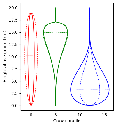
The code below generates a plot of the vertical shape profiles of the crowns for each stem. For each stem:

• the dashed line shows how the relative crown radius \(q(z)\) varies with height \(z\),

• the solid line shows how the actual crown radius \(r(z)\) varies with height, and

• the dotted horizontal line shows the height at which the maximum crown radius is found (\(z_{max}\)).

Note

The predictions of the equation for the relative radius \(q(z)\) are not limited to height values within the range of the actual height of a given stem (\(0 \leq z \leq H\)). This is critical for calculating behaviour with height across multiple stems when calculating canopy profiles for a community. The plot below includes predictions of \(q(z)\) below ground level and above stem height.

The get_crown_xy() helper function can be used to extract plotting structures for each stem within a CrownProfile that are restricted to actual valid heights for that stem and is demonstrated in the code below.

Show code cell source

Hide code cell source

fig, ax = plt.subplots(ncols=1)

# Find the maximum of the actual and relative maximum crown widths
max_relative_crown_radius = np.nanmax(crown_profiles.relative_crown_radius, axis=0)
max_crown_radius = np.nanmax(crown_profiles.crown_radius, axis=0)
stem_max_width = np.maximum(max_crown_radius, max_relative_crown_radius)


for pft_idx, offset, colour in zip((0, 1, 2), (0, 5, 12), ("r", "g", "b")):

    # Plot relative radius either side of offset
    stem_qz = crown_profiles.relative_crown_radius[:, pft_idx]
    ax.plot(stem_qz + offset, z, color=colour, linestyle="--", linewidth=1)
    ax.plot(-stem_qz + offset, z, color=colour, linestyle="--", linewidth=1)

    # Plot actual crown radius either side of offset
    stem_rz = crown_profiles.crown_radius[:, pft_idx]
    ax.plot(stem_rz + offset, z, color=colour)
    ax.plot(-stem_rz + offset, z, color=colour)

    # Add the height of maximum crown radius
    stem_rz_max = stem_max_width[pft_idx]

    ax.plot(
        [offset - stem_rz_max, offset + stem_rz_max],
        [allometry.crown_z_max[:, pft_idx]] * 2,
        color=colour,
        linewidth=1,
        linestyle=":",
    )

    ax.set_xlabel("Crown profile")
    ax.set_ylabel("Height above ground (m)")

ax.set_aspect(aspect=1)

We can also use the CanopyProfile class with a single row of heights to calculate the crown profile at the expected \(z_{max}\) and show that this matches the expected crown area from the T Model allometry.

# Calculate the crown profile across those heights for each PFT
z_max = flora.z_max_prop * stem_height
profile_at_zmax = CrownProfile(stem_traits=flora, stem_allometry=allometry, z=z_max)

print(profile_at_zmax.crown_radius**2 * np.pi)
print(allometry.crown_area)

[[ 1.32889447 18.82424746 48.5490359 ]]
[[ 1.32889447 18.82424746 48.5490359 ]]

/home/docs/checkouts/readthedocs.org/user_builds/pyrealm/checkouts/latest/pyrealm/core/experimental.py:72: ExperimentalFeatureWarning: 'Be aware that CrownProfile is an experimental feature of pyrealm and the implementation and API may change within major versions.'
  warn(qualname, ExperimentalFeatureWarning)

Visualising crown and leaf projected areas

We can also use the crown profile to generate projected area plots. This is hard to see using the PFTs defined above because they have very different crown areas, so the code below generates new profiles for a new set of PFTs that have similar crown area ratios but different shapes and gap fractions.

no_gaps_pft = PlantFunctionalType(
    name="no_gaps", h_max=20, m=1.5, n=1.5, f_g=0, ca_ratio=380
)
few_gaps_pft = PlantFunctionalType(
    name="few_gaps", h_max=20, m=1.5, n=4, f_g=0.1, ca_ratio=400
)
many_gaps_pft = PlantFunctionalType(
    name="many_gaps", h_max=20, m=4, n=1.5, f_g=0.3, ca_ratio=420
)

# Calculate allometries for each PFT at the same stem DBH
area_stem_dbh = np.array([0.4, 0.4, 0.4])
area_flora = Flora([no_gaps_pft, few_gaps_pft, many_gaps_pft])
area_allometry = StemAllometry(stem_traits=area_flora, at_dbh=area_stem_dbh)

# Calculate the crown profiles across those heights for each PFT
area_z = np.linspace(0, area_allometry.stem_height.max(), 201)[:, None]
area_crown_profiles = CrownProfile(
    stem_traits=area_flora, stem_allometry=area_allometry, z=area_z
)

/home/docs/checkouts/readthedocs.org/user_builds/pyrealm/checkouts/latest/pyrealm/core/experimental.py:72: ExperimentalFeatureWarning: 'Be aware that StemAllometry is an experimental feature of pyrealm and the implementation and API may change within major versions.'
  warn(qualname, ExperimentalFeatureWarning)

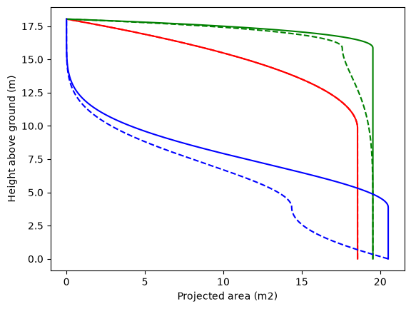
The plot below then shows how projected crown area (solid lines) and leaf area (dashed lines) change with height along the stem.

• The projected crown area increases from zero at the top of the crown until it reaches the maximum crown radius, at which point it remains constant down to ground level. The total crown areas differs for each stem because of the slightly different values used for the crown area ratio.

• The projected leaf area is very similar but leaf area is displaced towards the ground because of the crown gap fraction (f_g). Where f_g = 0 (the red line), the two lines are identical, but as f_g increases, more of the leaf area is displaced down within the crown.

Show code cell source

Hide code cell source

fig, ax = plt.subplots(ncols=1)

for pft_idx, offset, colour in zip((0, 1, 2), (0, 5, 10), ("r", "g", "b")):

    ax.plot(area_crown_profiles.projected_crown_area[:, pft_idx], area_z, color=colour)
    ax.plot(
        area_crown_profiles.projected_leaf_area[:, pft_idx],
        area_z,
        color=colour,
        linestyle="--",
    )
    ax.set_xlabel("Projected area (m2)")
    ax.set_ylabel("Height above ground (m)")

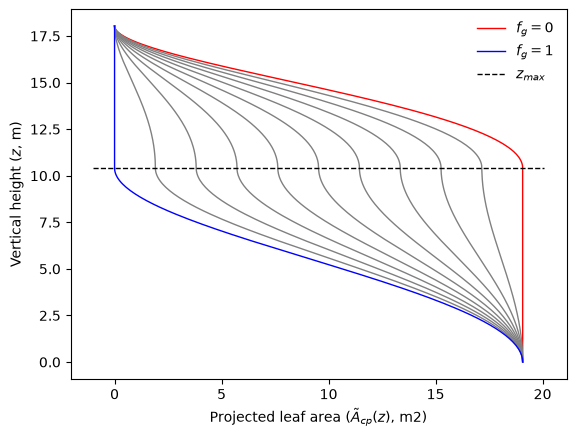
We can also generate predictions for a single PFT with varying crown gap fraction. In the plot below, note that all leaf area is above \(z_{max}\) when \(f_g=1\) and all leaf area is below \(z_{max}\) when \(f_g=0\).

Show code cell source

Hide code cell source

fig, ax = plt.subplots(ncols=1)

# Loop over f_g values
for f_g in np.linspace(0, 1, num=11):

    label = None
    colour = "gray"

    if f_g == 0:
        label = "$f_g=0$"
        colour = "red"
    elif f_g == 1:
        label = "$f_g=1$"
        colour = "blue"

    # Create a flora with a single PFT with current f_g and then generate a
    # stem allometry and crown profile
    flora_f_g = Flora(
        [PlantFunctionalType(name="example", h_max=20, m=2, n=2, f_g=f_g)]
    )
    allometry_f_g = StemAllometry(stem_traits=flora_f_g, at_dbh=np.array([0.4]))
    profile = CrownProfile(
        stem_traits=flora_f_g, stem_allometry=allometry_f_g, z=area_z
    )

    # Plot the projected leaf area with height
    ax.plot(profile.projected_leaf_area, area_z, color=colour, label=label, linewidth=1)

# Add a horizontal line for z_max
ax.plot(
    [-1, allometry_f_g.crown_area[0][0] + 1],
    [allometry_f_g.crown_z_max[0][0], allometry_f_g.crown_z_max[0][0]],
    linestyle="--",
    color="black",
    label="$z_{max}$",
    linewidth=1,
)

ax.set_ylabel(r"Vertical height ($z$, m)")
ax.set_xlabel(r"Projected leaf area ($\tilde{A}_{cp}(z)$, m2)")
_ = ax.legend(frameon=False)

Plotting tools for crown shapes

The get_crown_xy() function makes it easier to extract neat crown profiles from CrownProfile objects, for use in plotting crown data. The function takes a paired CrownProfile and StemAllometry and extracts a particular crown profile variable, and removes predictions for each stem that are outside of the stem range for that stem. It converts the data for each stem into coordinates that will plot as a complete two-sided crown outline. The returned value is a list with an entry for each stem in one of two formats.

• A pair of coordinate arrays: height and variable value.

• An single XY array with height and variable values in the columns, as used for example in matplotlib Patch objects.

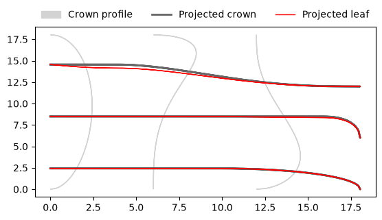
The code below uses this function to generate plotting data for the crown radius, projected crown radius and projected leaf radius. These last two variables do not have direct computational use - the cumulative projected area is what matters - but allow the projected variables to be visualised at the same scale as the crown radius.

# Set stem offsets for separating stems along the x axis
stem_offsets = np.array([0, 6, 12])

# Get the crown radius in XY format to plot as a polygon
crown_radius_as_xy = get_crown_xy(
    crown_profile=area_crown_profiles,
    stem_allometry=area_allometry,
    attr="crown_radius",
    stem_offsets=stem_offsets,
    as_xy=True,
)

# Get the projected crown and leaf radii to plot as lines
projected_crown_radius_xy = get_crown_xy(
    crown_profile=area_crown_profiles,
    stem_allometry=area_allometry,
    attr="projected_crown_radius",
    stem_offsets=stem_offsets,
)

projected_leaf_radius_xy = get_crown_xy(
    crown_profile=area_crown_profiles,
    stem_allometry=area_allometry,
    attr="projected_leaf_radius",
    stem_offsets=stem_offsets,
)

fig, ax = plt.subplots()

# Bundle the three plotting structures and loop over the three stems.
for cr_xy, (ch, cpr), (lh, lpr) in zip(
    crown_radius_as_xy, projected_crown_radius_xy, projected_leaf_radius_xy
):
    ax.add_patch(Polygon(cr_xy, color="lightgrey"))
    ax.plot(cpr, ch, color="0.4", linewidth=2)
    ax.plot(lpr, lh, color="red", linewidth=1)

ax.set_aspect(0.5)
_ = plt.legend(
    handles=[
        Patch(color="lightgrey", label="Crown profile"),
        Line2D([0], [0], label="Projected crown", color="0.4", linewidth=2),
        Line2D([0], [0], label="Projected leaf", color="red", linewidth=1),
    ],
    ncols=3,
    loc="upper center",
    bbox_to_anchor=(0.5, 1.15),
    frameon=False,
)