The T Model module

Run this notebook

Read the guide on setting up your computer to run Jupyter notebooks
Download this notebook as a Jupyter notebook.

import warnings

from matplotlib import pyplot as plt
import numpy as np
import pandas as pd

from pyrealm.core.experimental import ExperimentalFeatureWarning
from pyrealm.demography.flora import Flora
from pyrealm.demography.cohorts import create_cohorts, cohort_id_generator
from pyrealm.demography.tmodel import (
    StemAllocation,
    StemAllometry,
    GrowthIncrements,
    calculate_whole_crown_gpp,
)

warnings.filterwarnings(
    "ignore",
    category=ExperimentalFeatureWarning,
)

The T Model (Li et al., 2014) defines both the allometry of trees and a carbon allocation model for tree growth.

The allometry of a stem is driven by the diameter at breast height (DBH, metres) following a set of scaling relationships and defined stem traits for its plant functional type (PFT).

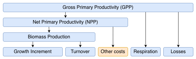
The carbon allocation for a stem partitions gross primary productivity (GPP) in respiration, turnover, growth and efficiency losses. The diagram below shows the allocation process:

Net primary productivity (NPP) is GPP less respiration, but also subject to yield losses. The T Model includes terms for foliage, stem and fine root respiration.
NPP is the carbon available for plant processes. The original T Model assumed all of the NPP went to biomass production, but the implementation in pyrealm allows users to modify NPP to apply other carbon costs, such as VOC emissions, root exudates or storage of non-structural carbohydrates.
Biomass production is then the fraction of NPP used to produce plant biomass. It has to account for turnover costs (branch, foliage and fine root) and then any remaining biomass production can be allocated to growth. Growth is calculated as the incremental increase in DBH that accounts for the required increase in stem, foliage and fine root masses, given the stem allometry.

GPP partition