Optimal \(\chi\) and leaf \(\ce{CO2}\)

Run this notebook

• Read the guide on setting up your computer to run Jupyter notebooks

• Download this notebook as a Jupyter notebook.

Once the key photosynthetic environment variables have been calculated, the next step is to estimate the following parameters:

• The ratio of carboxylation to transpiration cost factors (beta, \(\beta\)). In some approaches, this is taken as a fixed value, but other approaches apply penalties to \(\beta\) based on environmental conditions:

  • Two methods follow Lavergne et al. (2020) in using a statistical model of the variation of \(\beta\) with local soil moisture content (theta, \(\theta\))

  • The experimental rootzone stress approaches apply a user-provided local rootzone stress factor directly to a fixed value of \(\beta\) during the calculation of \(\xi\). This factor is not currently estimated within pyrealm.

• The value \(\chi = c_i/c_a\), which is the unitless ratio of leaf internal \(\ce{CO2}\) partial pressure (\(c_i\), Pa) to ambient \(\ce{CO2}\) partial pressure (\(c_a\), Pa).

• The parameter \(\xi\), which captures the sensitivity of \(\chi\) to vapour pressure deficit (VPD). This is a critical variable in the subdaily form of the P Model as it is expected to show slow responses to environmental change and should acclimate towards optimal behaviour on a time scale of days or weeks.

• \(\ce{CO2}\) limitation factors to both light assimilation (\(m_j\)) and carboxylation (\(m_c\)) along with their ratio (\(m_{joc} = m_j / m_c\)).

The optimal_chi module provides a range of methods for calculating optimal \(\chi\) and the other key values. The table below gives the method names, which are used to select a particular approach when fitting a P Model using the method_optchi argument.

In the background, those method names are used to select from a set of classes that implement the different calculations. Some of the examples below show these classes being used directly. The methods and classes built into pyrealm are shown below, but it is possible for users to add alternative methods for use within a P Model.

Method name	Method class
prentice14	OptimalChiPrentice14
c4	OptimalChiC4
c4_no_gamma	OptimalChiC4NoGamma
lavergne20_c3	OptimalChiLavergne20C3
lavergne20_c4	OptimalChiLavergne20C4
prentice14_rootzonestress	OptimalChiPrentice14RootzoneStress
c4_rootzonestress	OptimalChiC4RootzoneStress
c4_no_gamma_rootzonestress	OptimalChiC4NoGammaRootzoneStress

The sections and plots below show how optimal \(\chi\), \(m_j\) and \(m_c\) vary with differing methods and environmental conditions.

Show code cell source

Hide code cell source

from itertools import product

import numpy as np
from matplotlib import pyplot
from matplotlib.lines import Line2D

from pyrealm.pmodel.optimal_chi import OptimalChiPrentice14
from pyrealm.pmodel import PModelEnvironment
from pyrealm.pmodel.pmodel import PModel

# Create inputs for a temperature curve at:
# - two atmospheric pressures
# - two CO2 concentrations
# - two VPD values

n_pts = 31

tc_1d = np.linspace(-10, 40, n_pts)
patm_1d = np.array([101325, 80000])
vpd_1d = np.array([500, 2000])
co2_1d = np.array([280, 410])

tc_4d, patm_4d, vpd_4d, co2_4d = np.meshgrid(tc_1d, patm_1d, vpd_1d, co2_1d)

# Calculate the photosynthetic environment
pmodel_env = PModelEnvironment(
    tc=tc_4d, patm=patm_4d, vpd=vpd_4d, co2=co2_4d, fapar=1, ppfd=1
)


# A plotter function for a model
def plot_opt_chi(mod):

    # Create a list of combinations and line formats
    # (line col: PATM, style: CO2, marker used for VPD)

    idx_vals = {
        "vpd": zip([0, 1], vpd_1d),
        "patm": zip([0, 1], patm_1d),
        "co2": zip([0, 1], co2_1d),
    }

    idx_combos = list(product(*idx_vals.values()))
    line_formats = ["r-", "r--", "b-", "b--"] * 2

    # Create side by side subplots
    fig, (ax1, ax2, ax3) = pyplot.subplots(1, 3, figsize=(16, 5))

    # Loop over the variables
    for ax, var, label in (
        (ax1, "chi", "Optimal $\chi$"),
        (ax2, "mj", "$m_j$"),
        (ax3, "mc", "$m_c$"),
    ):

        # Get the variable to be plotted
        var_values = getattr(mod.optchi, var)

        # Plot line combinations
        for ((vdx, vvl), (pdx, pvl), (cdx, cvl)), lfmt in zip(idx_combos, line_formats):

            ax.plot(tc_1d, var_values[pdx, :, vdx, cdx], lfmt)

        # Annotate graph and force common y limits
        ax.set_title(f"Variation in {label}")
        ax.set_xlabel("Temperature °C")
        ax.set_ylabel(label)
        ax.set_ylim([-0.02, 1.02])

        # Add markers to note the two VPD inputs
        for vdx, mrkr in zip([0, 1], ["o", "^"]):

            mean_at_min_temp = var_values[:, 0, vdx, :].mean()
            ax.scatter(
                tc_1d[0] - 2,
                mean_at_min_temp,
                marker=mrkr,
                s=60,
                c="none",
                edgecolor="black",
            )

    # create a legend showing the combinations
    blnk = Line2D([], [], color="none")
    rd = Line2D([], [], linestyle="-", color="r")
    bl = Line2D([], [], linestyle="-", color="b")
    sld = Line2D([], [], linestyle="-", color="k")
    dsh = Line2D([], [], linestyle="--", color="k")
    circ = Line2D(
        [],
        [],
        marker="o",
        linestyle="",
        markersize=10,
        markeredgecolor="k",
        markerfacecolor="none",
    )
    trng = Line2D(
        [],
        [],
        marker="^",
        linestyle="",
        markersize=10,
        markeredgecolor="k",
        markerfacecolor="none",
    )

    ax1.legend(
        [blnk, blnk, blnk, rd, sld, circ, bl, dsh, trng],
        [
            "patm",
            "co2",
            "vpd",
            f"{patm_1d[0]} Pa",
            f"{co2_1d[0]} ppm",
            f"{vpd_1d[0]} Pa",
            f"{patm_1d[1]} Pa",
            f"{co2_1d[1]} ppm",
            f"{vpd_1d[1]} Pa",
        ],
        ncol=3,
        loc="upper left",
        frameon=False,
    )

    # pyplot.tight_layout();

<>:51: SyntaxWarning: invalid escape sequence '\c'
<>:51: SyntaxWarning: invalid escape sequence '\c'
/tmp/ipykernel_1467/2975497538.py:51: SyntaxWarning: invalid escape sequence '\c'
  (ax1, "chi", "Optimal $\chi$"),

The prentice14 method

This C3 method follows the approach detailed in Prentice et al. (2014), see OptimalChiPrentice14 for details.

Show code cell source

Hide code cell source

# Run the P Model and plot predictions
pmodel_c3 = PModel(pmodel_env, method_optchi="prentice14")
plot_opt_chi(pmodel_c3)

/home/docs/checkouts/readthedocs.org/user_builds/pyrealm/checkouts/latest/pyrealm/pmodel/pmodel.py:481: UserWarning: 
    Pyrealm 2.0.0 uses a new default for the quantum yield of photosynthesis (phi0=1/8).
    You may need to change settings to duplicate results from pyrealm 1.0.0.
            
  warn(

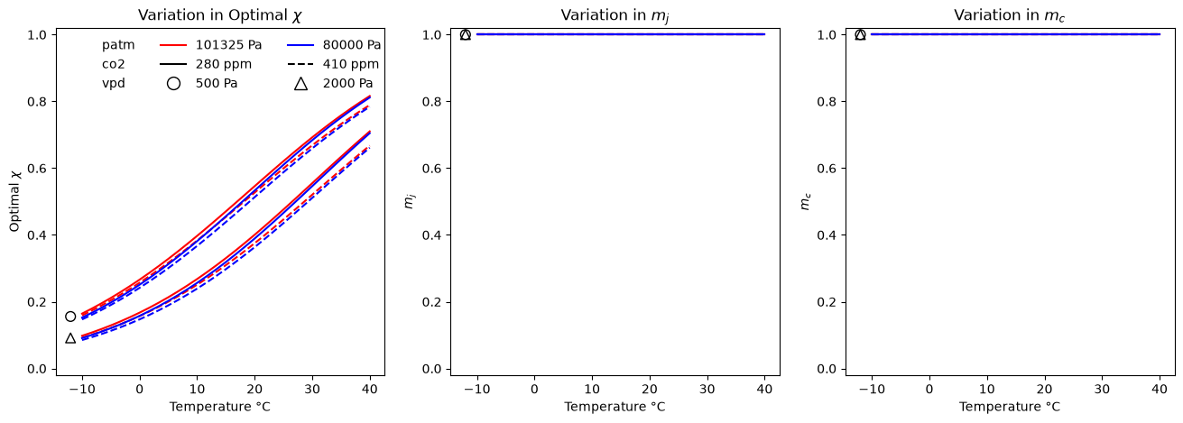
The c4 method

This C4 method follows the approach detailed in Prentice et al. (2014), but uses a C4 specific version of the unit cost ratio (\(\beta\)). It also sets \(m_j = m_c = 1\). See OptimalChiC4 for details.

Show code cell source

Hide code cell source

# Run the P Model and plot predictions
pmodel_c4 = PModel(pmodel_env, method_optchi="c4")
plot_opt_chi(pmodel_c4)

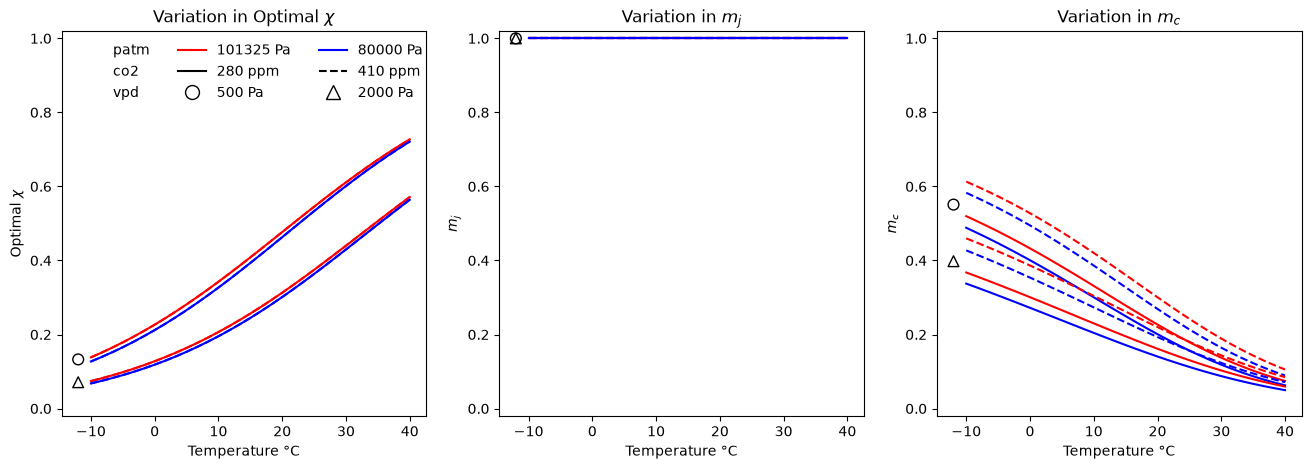
The c4_no_gamma method

This method drops terms from the approach given in Prentice et al. (2014) to reflect the assumption that photorespiration (\(\Gamma^\ast\)) is negligible in C4 photosynthesis. It uses the same \(\beta\) estimate as OptimalChiC4 and also also sets \(m_j = 1\), but \(m_c\) is calculated as in OptimalChiPrentice14. See OptimalChiC4NoGamma() for details.

Show code cell source

Hide code cell source

# Run the P Model and plot predictions
pmodel_c4 = PModel(pmodel_env, method_optchi="c4_no_gamma")
plot_opt_chi(pmodel_c4)

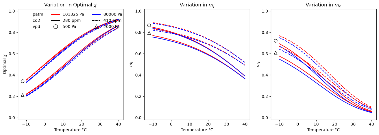
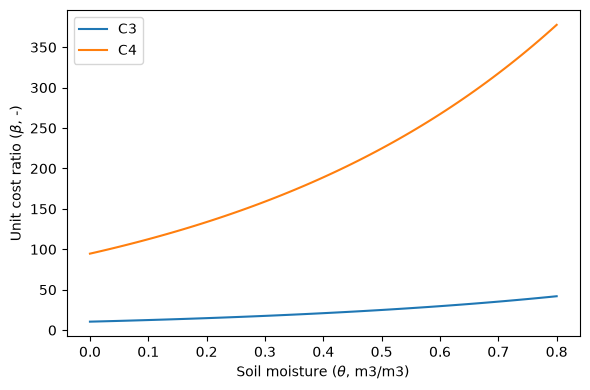
The lavergne20_c3 and lavergne20_c4 methods

These methods follow the approach detailed in Lavergne et al. (2020), which fitted an empirical model of \(\beta\) for C3 plants as a function of volumetric soil moisture (\(\theta\), m3/m3), using data from leaf gas exchange measurements. The C4 method takes the same approach but with modified empirical parameters giving predictions of \(\beta_{C3} = 9 \times \beta_{C4}\). Following the approach of OptimalChiC4NoGamma, \(m_c\) is calculated but \(m_j=1\).

Warning

Note that Lavergne et al. (2020) found no relationship between C4 \(\beta\) values and soil moisture in leaf gas exchange data The OptimalChiLavergne20C4 method is an experimental feature - see the documentation for the OptimalChiLavergne20C4 and OptimalChiC4 methods for the theoretical rationale.

Variation in \(\beta\) with soil moisture

The calculation details are provided in the description of the OptimalChiLavergne20C3 method, but the variation in \(\beta\) with \(\theta\) is shown below.

Show code cell source

Hide code cell source

# Theta is required for the calculation of beta
from pyrealm.pmodel.optimal_chi import OptimalChiLavergne20C3, OptimalChiLavergne20C4

pmodel_env_theta_range = PModelEnvironment(
    tc=25, patm=101325, vpd=0, co2=400, fapar=1, ppfd=1, theta=np.linspace(0, 0.8, 81)
)
opt_chi_lavergne20_c3 = OptimalChiLavergne20C3(pmodel_env_theta_range)
opt_chi_lavergne20_c4 = OptimalChiLavergne20C4(pmodel_env_theta_range)

# Plot the predictions
fig, ax1 = pyplot.subplots(1, 1, figsize=(6, 4))
ax1.plot(pmodel_env_theta_range.theta, opt_chi_lavergne20_c4.beta, label="C3")
ax1.plot(pmodel_env_theta_range.theta, opt_chi_lavergne20_c3.beta, label="C4")
ax1.set_xlabel(r"Soil moisture ($\theta$, m3/m3)")
ax1.set_ylabel(r"Unit cost ratio ($\beta$, -)")
ax1.legend()
pyplot.tight_layout()

/home/docs/checkouts/readthedocs.org/user_builds/pyrealm/checkouts/latest/pyrealm/core/experimental.py:72: ExperimentalFeatureWarning: 'Be aware that OptimalChiLavergne20C4 is an experimental feature of pyrealm and the implementation and API may change within major versions.'
  warn(qualname, ExperimentalFeatureWarning)

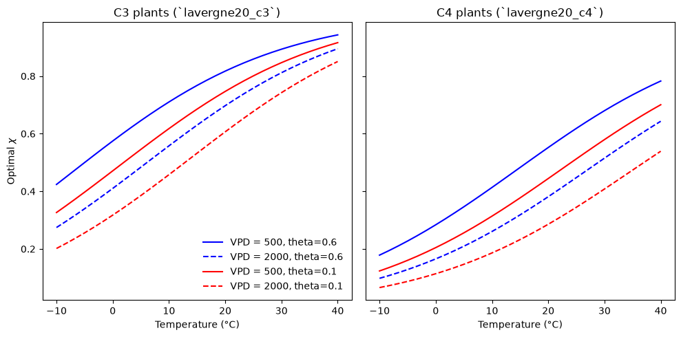
Estimation of optimal \(\chi\)

The plots below show the impacts on optimal \(\chi\) across a temperature gradient for two values of VPD and soil moisture, with constant atmospheric pressure (101325 Pa) and CO2 (280 ppm).

Show code cell source

Hide code cell source

# Environments with high and low soil moisture
theta_hi = 0.6
theta_lo = 0.1
pmodel_env_hi = PModelEnvironment(
    tc=tc_4d, patm=patm_4d, vpd=vpd_4d, co2=co2_4d, fapar=1, ppfd=1, theta=theta_hi
)
pmodel_env_lo = PModelEnvironment(
    tc=tc_4d, patm=patm_4d, vpd=vpd_4d, co2=co2_4d, fapar=1, ppfd=1, theta=theta_lo
)

# Run the P Model and plot predictions
chi_lavc3_hi = OptimalChiLavergne20C3(pmodel_env_hi)
chi_lavc4_hi = OptimalChiLavergne20C4(pmodel_env_hi)
chi_lavc3_lo = OptimalChiLavergne20C3(pmodel_env_lo)
chi_lavc4_lo = OptimalChiLavergne20C4(pmodel_env_lo)

fig, (ax1, ax2) = pyplot.subplots(1, 2, figsize=(10, 5), sharey=True)

ax1.plot(
    tc_1d,
    chi_lavc3_hi.chi[0, :, 0, 0],
    "b-",
    label=f"VPD = {vpd_1d[0]}, theta={theta_hi}",
)
ax1.plot(
    tc_1d,
    chi_lavc3_hi.chi[0, :, 1, 0],
    "b--",
    label=f"VPD = {vpd_1d[1]}, theta={theta_hi}",
)
ax1.plot(
    tc_1d,
    chi_lavc3_lo.chi[0, :, 0, 0],
    "r-",
    label=f"VPD = {vpd_1d[0]}, theta={theta_lo}",
)
ax1.plot(
    tc_1d,
    chi_lavc3_lo.chi[0, :, 1, 0],
    "r--",
    label=f"VPD = {vpd_1d[1]}, theta={theta_lo}",
)
ax1.set_title(f"C3 plants (`lavergne20_c3`)")
ax1.set_ylabel(r"Optimal $\chi$")
ax1.set_xlabel("Temperature (°C)")
ax1.legend(frameon=False)

ax2.plot(tc_1d, chi_lavc4_hi.chi[0, :, 0, 0], "b-")
ax2.plot(tc_1d, chi_lavc4_hi.chi[0, :, 1, 0], "b--")
ax2.plot(tc_1d, chi_lavc4_lo.chi[0, :, 0, 0], "r-")
ax2.plot(tc_1d, chi_lavc4_lo.chi[0, :, 1, 0], "r--")
ax2.set_title(f"C4 plants (`lavergne20_c4`)")
ax2.set_xlabel("Temperature (°C)")

pyplot.tight_layout()

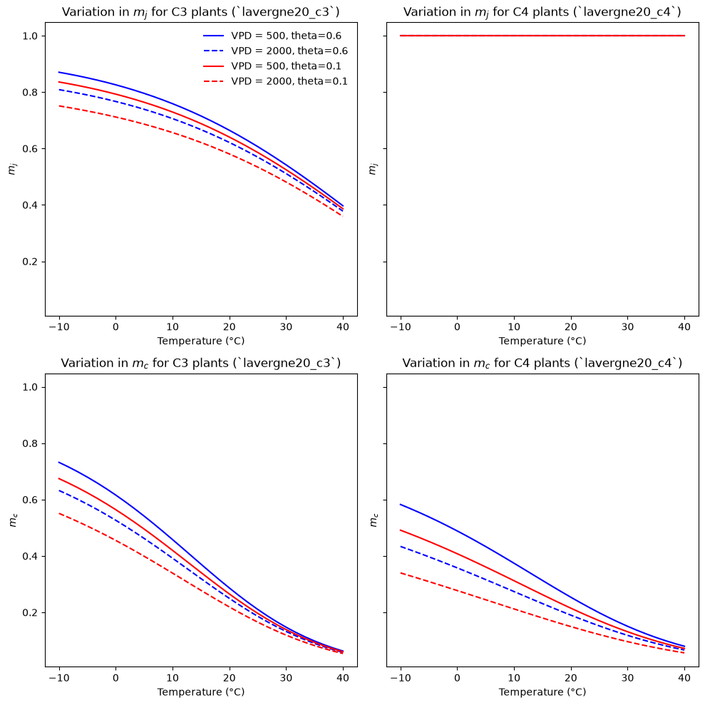
\(m_j\) and \(m_c\)

The plots below illustrate the impact of temperature and \(\theta\) on \(m_j\) and \(m_c\), again with constant atmospheric pressure (101325 Pa) and CO2 (280 ppm).

Show code cell source

Hide code cell source

fig, ((ax1, ax3), (ax2, ax4)) = pyplot.subplots(2, 2, figsize=(10, 10), sharey=True)

ax1.plot(
    tc_1d,
    chi_lavc3_hi.mj[0, :, 0, 0],
    "b-",
    label=f"VPD = {vpd_1d[0]}, theta={theta_hi}",
)
ax1.plot(
    tc_1d,
    chi_lavc3_hi.mj[0, :, 1, 0],
    "b--",
    label=f"VPD = {vpd_1d[1]}, theta={theta_hi}",
)
ax1.plot(
    tc_1d,
    chi_lavc3_lo.mj[0, :, 0, 0],
    "r-",
    label=f"VPD = {vpd_1d[0]}, theta={theta_lo}",
)
ax1.plot(
    tc_1d,
    chi_lavc3_lo.mj[0, :, 1, 0],
    "r--",
    label=f"VPD = {vpd_1d[1]}, theta={theta_lo}",
)
ax1.set_title(f"Variation in $m_j$ for C3 plants (`lavergne20_c3`)")
ax1.set_ylabel(r"$m_j$")
ax1.set_xlabel("Temperature (°C)")
ax1.legend(frameon=False)

ax2.plot(tc_1d, chi_lavc3_hi.mc[0, :, 0, 0], "b-")
ax2.plot(tc_1d, chi_lavc3_hi.mc[0, :, 1, 0], "b--")
ax2.plot(tc_1d, chi_lavc3_lo.mc[0, :, 0, 0], "r-")
ax2.plot(tc_1d, chi_lavc3_lo.mc[0, :, 1, 0], "r--")
ax2.set_title(f"Variation in $m_c$ for C3 plants (`lavergne20_c3`)")
ax2.set_ylabel(r"$m_c$")
ax2.set_xlabel("Temperature (°C)")

ax3.plot(
    tc_1d,
    chi_lavc4_hi.mj[0, :, 0, 0],
    "b-",
    label=f"VPD = {vpd_1d[0]}, theta={theta_hi}",
)
ax3.plot(
    tc_1d,
    chi_lavc4_hi.mj[0, :, 1, 0],
    "b--",
    label=f"VPD = {vpd_1d[1]}, theta={theta_hi}",
)
ax3.plot(
    tc_1d,
    chi_lavc4_lo.mj[0, :, 0, 0],
    "r-",
    label=f"VPD = {vpd_1d[0]}, theta={theta_lo}",
)
ax3.plot(
    tc_1d,
    chi_lavc4_lo.mj[0, :, 1, 0],
    "r--",
    label=f"VPD = {vpd_1d[1]}, theta={theta_lo}",
)
ax3.set_title(f"Variation in $m_j$ for C4 plants (`lavergne20_c4`)")
ax3.set_ylabel(r"$m_j$")
ax3.set_xlabel("Temperature (°C)")

ax4.plot(tc_1d, chi_lavc4_hi.mc[0, :, 0, 0], "b-")
ax4.plot(tc_1d, chi_lavc4_hi.mc[0, :, 1, 0], "b--")
ax4.plot(tc_1d, chi_lavc4_lo.mc[0, :, 0, 0], "r-")
ax4.plot(tc_1d, chi_lavc4_lo.mc[0, :, 1, 0], "r--")
ax4.set_title(f"Variation in $m_c$ for C4 plants (`lavergne20_c4`)")
ax4.set_ylabel(r"$m_c$")
ax4.set_xlabel("Temperature (°C)")

pyplot.tight_layout()

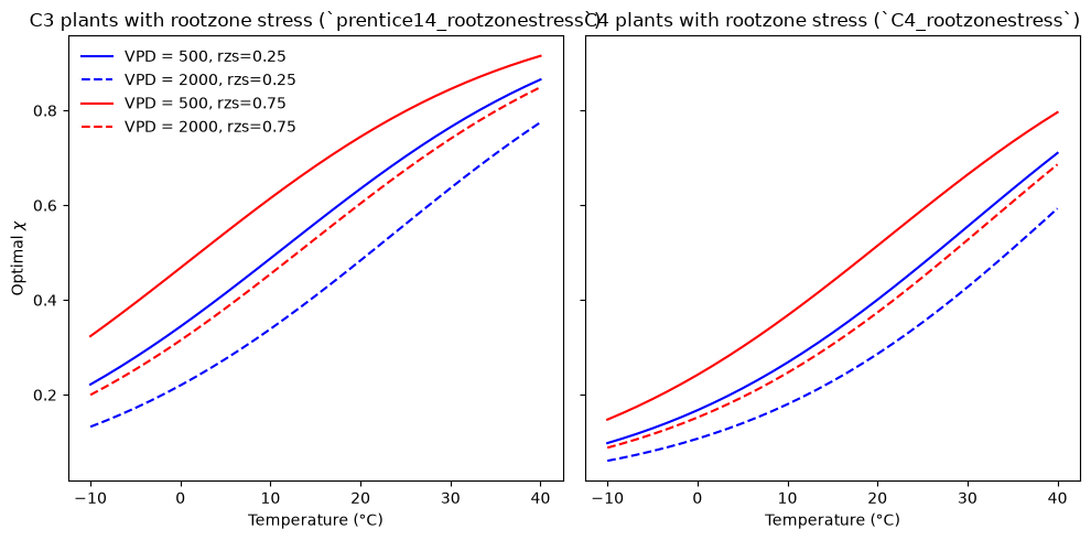
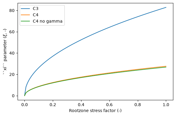
The rootzone stress methods

These are experimental approaches that take a rootzone stress factor and use this to directly penalise \(\beta\) in calculating \(\xi\) and hence \(\chi\) and other variables. The approach is being developed by Rodolfo Nobrega and the calculation of the factor itself is not yet included in pyrealm.

Variation in \(\beta\) with rootzone stress

The calculation details are provided in the description of the following three methods but the variation in \(\beta\) with rootzone stress is shown below.

• OptimalChiPrentice14RootzoneStress

• OptimalChiC4RootzoneStress

• OptimalChiC4NoGammaRootzoneStress

Show code cell source

Hide code cell source

from pyrealm.pmodel.optimal_chi import (
    OptimalChiPrentice14RootzoneStress,
    OptimalChiC4RootzoneStress,
    OptimalChiC4NoGammaRootzoneStress,
)

# Rootzone stress is required for the calculation of beta
pmodel_env_rootzonestress = PModelEnvironment(
    tc=np.repeat(25, 101),
    patm=np.repeat(101325, 101),
    vpd=np.repeat(1000, 101),
    co2=np.repeat(400, 101),
    fapar=np.repeat(1, 101),
    ppfd=np.repeat(1, 101),
    rootzonestress=np.linspace(0, 1, 101),
)

# Estimate using the 3 different methods
opt_chi_prentice14_rzs = OptimalChiPrentice14RootzoneStress(pmodel_env_rootzonestress)
opt_chi_c4_rzs = OptimalChiC4RootzoneStress(pmodel_env_rootzonestress)
opt_chi_c4_no_gamma_rzs = OptimalChiC4NoGammaRootzoneStress(pmodel_env_rootzonestress)

# Plot the predictions
fig, ax1 = pyplot.subplots(1, 1, figsize=(6, 4))
ax1.plot(
    pmodel_env_rootzonestress.rootzonestress, opt_chi_prentice14_rzs.xi, label="C3"
)
ax1.plot(pmodel_env_rootzonestress.rootzonestress, opt_chi_c4_rzs.xi, label="C4")
ax1.plot(
    pmodel_env_rootzonestress.rootzonestress,
    opt_chi_c4_no_gamma_rzs.xi,
    label="C4 no gamma",
)
ax1.set_xlabel(r"Rootzone stress factor (-)")
ax1.set_ylabel(r"``xi`` parameter ($\xi$, -)")
ax1.legend()
pyplot.tight_layout()

/home/docs/checkouts/readthedocs.org/user_builds/pyrealm/checkouts/latest/pyrealm/core/experimental.py:72: ExperimentalFeatureWarning: 'Be aware that OptimalChiPrentice14RootzoneStress is an experimental feature of pyrealm and the implementation and API may change within major versions.'
  warn(qualname, ExperimentalFeatureWarning)
/home/docs/checkouts/readthedocs.org/user_builds/pyrealm/checkouts/latest/pyrealm/pmodel/optimal_chi.py:354: RuntimeWarning: invalid value encountered in divide
  self.mjoc = self.mj / self.mc
/home/docs/checkouts/readthedocs.org/user_builds/pyrealm/checkouts/latest/pyrealm/core/experimental.py:72: ExperimentalFeatureWarning: 'Be aware that OptimalChiC4NoGammaRootzoneStress is an experimental feature of pyrealm and the implementation and API may change within major versions.'
  warn(qualname, ExperimentalFeatureWarning)
/home/docs/checkouts/readthedocs.org/user_builds/pyrealm/checkouts/latest/pyrealm/pmodel/optimal_chi.py:815: RuntimeWarning: divide by zero encountered in divide
  self.mjoc = self.mj / self.mc

Estimation of optimal \(\chi\) with rootzone stress

The plots below show the impacts on optimal \(\chi\) across a temperature gradient for two values of VPD and rootzone stress, with constant atmospheric pressure (101325 Pa) and CO2 (280 ppm).

Show code cell source

Hide code cell source

# Environments with high and low rootzone stress
rzs_low = 0.75
rzs_high = 0.25

pmodel_env_hi = PModelEnvironment(
    tc=tc_4d,
    patm=101325,
    vpd=vpd_4d,
    co2=co2_4d,
    fapar=1,
    ppfd=1,
    rootzonestress=rzs_high,
)
pmodel_env_lo = PModelEnvironment(
    tc=tc_4d,
    patm=patm_4d,
    vpd=vpd_4d,
    co2=co2_4d,
    fapar=1,
    ppfd=1,
    rootzonestress=rzs_low,
)

# Run the P Model and plot predictions
chi_lavc3_hi = OptimalChiPrentice14RootzoneStress(pmodel_env_hi)
chi_lavc4_hi = OptimalChiC4RootzoneStress(pmodel_env_hi)
chi_lavc3_lo = OptimalChiPrentice14RootzoneStress(pmodel_env_lo)
chi_lavc4_lo = OptimalChiC4RootzoneStress(pmodel_env_lo)

fig, (ax1, ax2) = pyplot.subplots(1, 2, figsize=(10, 5), sharey=True)

ax1.plot(
    tc_1d,
    chi_lavc3_hi.chi[0, :, 0, 0],
    "b-",
    label=f"VPD = {vpd_1d[0]}, rzs={rzs_high}",
)
ax1.plot(
    tc_1d,
    chi_lavc3_hi.chi[0, :, 1, 0],
    "b--",
    label=f"VPD = {vpd_1d[1]}, rzs={rzs_high}",
)
ax1.plot(
    tc_1d,
    chi_lavc3_lo.chi[0, :, 0, 0],
    "r-",
    label=f"VPD = {vpd_1d[0]}, rzs={rzs_low}",
)
ax1.plot(
    tc_1d,
    chi_lavc3_lo.chi[0, :, 1, 0],
    "r--",
    label=f"VPD = {vpd_1d[1]}, rzs={rzs_low}",
)
ax1.set_title(f"C3 plants with rootzone stress (`prentice14_rootzonestress`)")
ax1.set_ylabel(r"Optimal $\chi$")
ax1.set_xlabel("Temperature (°C)")
ax1.legend(frameon=False)

ax2.plot(tc_1d, chi_lavc4_hi.chi[0, :, 0, 0], "b-")
ax2.plot(tc_1d, chi_lavc4_hi.chi[0, :, 1, 0], "b--")
ax2.plot(tc_1d, chi_lavc4_lo.chi[0, :, 0, 0], "r-")
ax2.plot(tc_1d, chi_lavc4_lo.chi[0, :, 1, 0], "r--")
ax2.set_title(f"C4 plants with rootzone stress (`C4_rootzonestress`)")
ax2.set_xlabel("Temperature (°C)")

pyplot.tight_layout()