Phenology
Run this notebook
Read the guide on setting up your computer to run Jupyter notebooks
Download
this notebookas a Jupyter notebook.
The Phenology class is used to generate
daily predictions of leaf area index (LAI). The approach requires:
daily estimates of total potential assimilation (\(A_0\)), typically estimated using a P Model, and
estimates of the annual maximum LAI for sites
Phenology methods
Methods to calculate daily LAI have two steps:
Converting daily \(A_0\) into steady state daily LAI (\(L_s\)), which is the LAI that would be possible if leaf creation was instantaneous.
Calculating a lagged value for realised LAI (\(L_r\)), capturing the time taken to actually grow leaves.
There are currently two methods implemented in pyrealm, selected by the method
argument to Phenology.
The zhou method
This method follows the approach of :cite:zhou:2025a. The details of the calculation
are provided in the documentation of the
PhenologyMethodZhou class, but in summary:
A scaling factor \(m\) is calculated that represents the fraction of daily potential assimilation (\(A_{d0}\)) allocated to leaf growth, using a parameterised function that accounts for seasonal patterns in canopy generation.
A daily allocation to leaf growth (\(\mu\)) is calculated as \(\mu = m \cdot A_{d0}\).
The steady state leaf area index is calculated using the Lambert W function to back calculate LAI under Beer’s law.
The realised leaf area index is calculated using a running exponential weighted average along the time series of steady state LAI estimates.
The zhu method
This method follows the approach of :cite:zhu:2026a. The details of the calculation
are provided in the documentation of the
PhenologyMethodZhu class, but in summary:
The scaling factor \(m\) is estimated simply as the ratio of maximum LAI to the 95% quantile value of \(A_{d0}\). This is essentially maximum LAI over maximum daily assimilation but controls for outliers.
The steady state LAI is then calculated simply as \(L_s = m \cdot A_{d0}\).
The realised LAI for a given day is calculated as the weighted average over a window of the preceding N days. The value of N is calculated as a parameterised function of site-specific aridity expressed as AET/PET.
By default, the method conditions estimates of \(L_r\) at the start of the time series by assuming stationarity: it prepends data from the end of the first year to provide the required N days of preceding data.
Example calculations
As with estimating maximum fAPAR, the examples below uses a
time series of half hourly data from the DE_Gri Fluxnet
site from 2004 to 2014 that has been
resampled to show different workflows for calculating annual maximum fAPAR. The
different workflows use some site specific scalar values, loaded in the following code.
import os

os.environ["PYREALM_USE_LOCAL_DATA"] = "SET"
# Load site data
site_data_path = get_pyrealm_data("phenology/inputs/source/DE-GRI_site_data.json")

with open(site_data_path) as json_src:
    site_data = json.load(json_src)
Direct calculation for daily assimilation values
Calculating phenology directly from a time series of daily total potential assimilation requires:
a
FaparLimitationinstance that provides maximum annual fAPAR and LAI for sites, andthe dates of the daily observations to match daily values to year.
The code below creates a FaparLimitation instance for 11 years of data from the
DE_Gri fluxnet site.
# Load annual estimates
annual_data_path = get_pyrealm_data("phenology/inputs/subdaily/annual_inputs.csv")
annual_data = pd.read_csv(annual_data_path)
annual_data["time"] = annual_data["year"].to_numpy().astype(str).astype("datetime64[Y]")

faparlim = FaparLimitation(
    method="cai",
    annual_total_potential_gpp=annual_data["annual_total_A0"].to_numpy(),
    annual_mean_ca=annual_data["annual_mean_ca_in_GS"].to_numpy(),
    annual_mean_chi=annual_data["annual_mean_chi_in_GS"].to_numpy(),
    annual_mean_vpd=annual_data["annual_mean_VPD_in_GS"].to_numpy(),
    annual_total_precip=annual_data["annual_precip_molar"].to_numpy(),
    annual_growing_season_length=annual_data["N_growing_days"].to_numpy(),
    years=annual_data["time"].to_numpy().astype("datetime64[Y]"),
    aridity_index=np.array([site_data["AI_from_cruts"]]),
)
/home/docs/checkouts/readthedocs.org/user_builds/pyrealm/checkouts/latest/pyrealm/core/experimental.py:72: ExperimentalFeatureWarning: 'Be aware that FaparLimitation is an experimental feature of pyrealm and the implementation and API may change within major versions.'
  warn(qualname, ExperimentalFeatureWarning)
We can then load estimates of daily total potential assimilation, get the date times of
the observation and calculate the time series of LAI. The code below fits LAI using both
methods: note that method="zhu" requires site specific estimates of the climatological
AET/PET ratio and also requires a specified spin up length used to condition initial
estimates of LAI.
# Load daily assimilation data
daily_assimilation_path = get_pyrealm_data(
    "phenology/inputs/subdaily/daily_assimilation.csv"
)
daily_assimilation = pd.read_csv(daily_assimilation_path)
daily_assimilation["time"] = pd.to_datetime(daily_assimilation["time"])

# Calculate LAI
phenology_direct_zhou = Phenology(
    method="zhou",
    fapar_limitation=faparlim,
    daily_potential_assimilation=daily_assimilation["daily_A0"].to_numpy(),
    datetimes=daily_assimilation["time"].to_numpy(),
)


# Calculate LAI
phenology_direct_zhu = Phenology(
    method="zhu",
    fapar_limitation=faparlim,
    daily_potential_assimilation=daily_assimilation["daily_A0"].to_numpy(),
    datetimes=daily_assimilation["time"].to_numpy(),
    aet_pet_ratio=np.array([site_data["aet_pet_ratio"]]),
    spinup_length=365,
)
/home/docs/checkouts/readthedocs.org/user_builds/pyrealm/checkouts/latest/pyrealm/core/experimental.py:72: ExperimentalFeatureWarning: 'Be aware that Phenology is an experimental feature of pyrealm and the implementation and API may change within major versions.'
  warn(qualname, ExperimentalFeatureWarning)
/home/docs/checkouts/readthedocs.org/user_builds/pyrealm/checkouts/latest/pyrealm/phenology/phenology.py:397: RuntimeWarning: divide by zero encountered in divide
  realised_lai[full_idx] = numerator / denominator
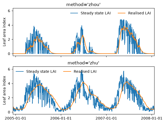
The plots show the resulting predicted steady state and realised LAI for two years of data. Because the underlying data in this example uses the original half hourly FluxNET data, there are large day to day variations in potential assimilation. This is why the steady state LAI changes so rapidly; the realised LAI smooths out these rapid fluctuations.
fig, axes = plt.subplots(nrows=2, sharex=True, sharey=True)

for ax, pheno, method in zip(
    axes,
    (phenology_direct_zhou, phenology_direct_zhu),
    ("zhou", "zhu"),
):
    ax.plot(pheno.datetimes, pheno.steady_state_lai, label="Steady state LAI")
    ax.plot(pheno.datetimes, pheno.realised_lai, label="Realised LAI")
    ax.set_ylabel("Leaf area index")
    ax.legend(frameon=False, ncol=2)
    ax.set_title(f"method='{method}'")
    ax.set_xlim(np.datetime64("2004-12-10"), np.datetime64("2008-01-21"))
    ax.set_xticks(
        np.arange(np.datetime64("2005"), np.datetime64("2009"), np.timedelta64(1, "Y"))
    )

plt.tight_layout()
Calculation from a fitted PModel
As with calculating annual maximum fAPAR, in most cases
the inputs for estimating daily LAI will come from a P Model. The
Phenology.from_pmodel
method can be used to automatically estimate daily assimilation from a P Model.
The estimation process is different for subdaily and standard P Models:
For a standard P Model, which typically use weekly to monthly observations, daily assimilation is estimated using linear interpolation between observation dates.
For subdaily P Models, the mean daily GPP is calculated from all the observations within each day.
In both cases, the resulting GPP is then converted from units of gC m-2 s-1 to mol C m-2 day-1. The examples below show a full workflow for calculating LAI using P Model
inputs.
Fortnightly data
This example uses fortnightly data. First the code calculates a P Model from the inputs.
# Load data and fit a PModel
fortnightly_data_path = get_pyrealm_data(
    "phenology/inputs/fortnightly/pmodel_inputs.csv"
)
fortnightly_data = pd.read_csv(fortnightly_data_path)

fortnightly_pmodel_env = PModelEnvironment(
    tc=fortnightly_data["tc"].to_numpy(),
    patm=fortnightly_data["patm"].to_numpy(),
    co2=fortnightly_data["co2"].to_numpy(),
    vpd=fortnightly_data["vpd"].to_numpy(),
    ppfd=fortnightly_data["ppfd"].to_numpy(),
    fapar=fortnightly_data["fapar"].to_numpy(),
)

fortnightly_pmodel = PModel(env=fortnightly_pmodel_env)

datetimes = fortnightly_data["time"].to_numpy(dtype="datetime64[D]")
/home/docs/checkouts/readthedocs.org/user_builds/pyrealm/checkouts/latest/pyrealm/pmodel/pmodel.py:481: UserWarning:
            The default value for quantum yield of photosynthesis (phi0=1/8) has changed
            since pyrealm 1.0.0. You may need to change settings to duplicate results
            from pyrealm 1.0.0.

  warn(
Next, calculate fAPAR and LAI limitation using each of the two available methods:
annual_faparlim_fortnightly_cai = FaparLimitation.from_pmodel(
    method="cai",
    pmodel=fortnightly_pmodel,
    datetimes=datetimes,
    growing_season=fortnightly_data["tc"].to_numpy() > 0,
    precip=fortnightly_data["precip_molar"].to_numpy(),
    aridity_index=np.array([site_data["AI_from_cruts"]]),
)

annual_faparlim_fortnightly_zhu = FaparLimitation.from_pmodel(
    method="zhu",
    pmodel=fortnightly_pmodel,
    datetimes=datetimes,
    growing_season=fortnightly_data["tc"].to_numpy() > 0,
    precip=fortnightly_data["precip_molar"].to_numpy(),
)
/home/docs/checkouts/readthedocs.org/user_builds/pyrealm/checkouts/latest/pyrealm/core/experimental.py:72: ExperimentalFeatureWarning: 'Be aware that FaparLimitation is an experimental feature of pyrealm and the implementation and API may change within major versions.'
  warn(qualname, ExperimentalFeatureWarning)
Now we can use the Phenology.from_pmodel method to automatically estimate daily
assimilation from the P Model. Note that using the method with a standard P Model again
requires datetimes to map the observations onto years and to interpolate GPP to daily
values.
phenology_fortnightly_zhou = Phenology.from_pmodel(
    method="zhou",
    pmodel=fortnightly_pmodel,
    datetimes=datetimes,
    fapar_limitation=annual_faparlim_fortnightly_cai,
)

phenology_fortnightly_zhu = Phenology.from_pmodel(
    method="zhu",
    pmodel=fortnightly_pmodel,
    datetimes=datetimes,
    fapar_limitation=annual_faparlim_fortnightly_zhu,
    aet_pet_ratio=np.array([site_data["aet_pet_ratio"]]),
    spinup_length=365,
)
/home/docs/checkouts/readthedocs.org/user_builds/pyrealm/checkouts/latest/pyrealm/core/experimental.py:72: ExperimentalFeatureWarning: 'Be aware that Phenology is an experimental feature of pyrealm and the implementation and API may change within major versions.'
  warn(qualname, ExperimentalFeatureWarning)
/home/docs/checkouts/readthedocs.org/user_builds/pyrealm/checkouts/latest/pyrealm/phenology/phenology.py:397: RuntimeWarning: divide by zero encountered in divide
  realised_lai[full_idx] = numerator / denominator
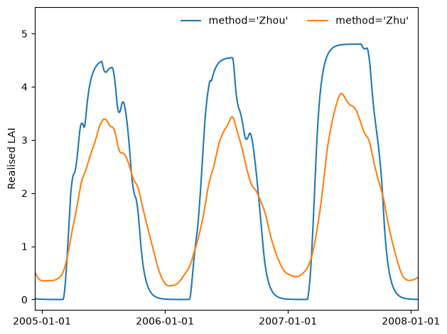
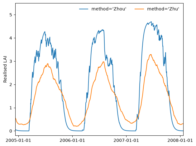
The plot below then shows the predictions of realised LAI from the two methods.
plt.plot(
    phenology_fortnightly_zhou.datetimes,
    phenology_fortnightly_zhou.realised_lai,
    label="method='Zhou'",
)
plt.plot(
    phenology_fortnightly_zhu.datetimes,
    phenology_fortnightly_zhu.realised_lai,
    label="method='Zhu'",
)
plt.legend(frameon=False, ncol=2)
plt.ylim(-0.2, 5.5)
plt.ylabel("Realised LAI")
plt.xlim(np.datetime64("2004-12-10"), np.datetime64("2008-01-21"))
plt.xticks(
    np.arange(np.datetime64("2005"), np.datetime64("2009"), np.timedelta64(1, "Y"))
)

plt.tight_layout()
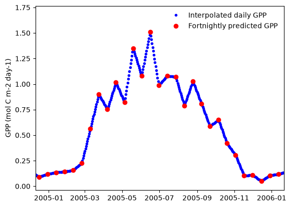
Just to show the workings of the method, the plot below superimposes the original estimated fortnightly GPP estimates and the daily interpolated values used to calculate LAI.
plt.plot(
    phenology_fortnightly_zhou.datetimes,
    phenology_fortnightly_zhou.daily_potential_assimilation,
    "b.",
    label="Interpolated daily GPP",
)
plt.plot(
    datetimes,
    fortnightly_pmodel.gpp * fortnightly_pmodel.gpp_conversion_factor,
    "ro",
    label="Fortnightly predicted GPP",
)
plt.ylabel("GPP (mol C m-2 day-1)")
plt.xlim(np.datetime64("2004-12-10"), np.datetime64("2006-01-21"))
_ = plt.legend(frameon=False)
Subdaily data
The code below shows the same workflow but instead using subdaily inputs and a subdaily P Model.
# Load subdaily data
subdaily_data_path = get_pyrealm_data("phenology/inputs/subdaily/pmodel_inputs.csv")
subdaily_data = pd.read_csv(subdaily_data_path)

# Fit a Subdaily P Model
subdaily_pmodel_env = PModelEnvironment(
    tc=subdaily_data["tc"].to_numpy(),
    patm=subdaily_data["patm"].to_numpy(),
    co2=subdaily_data["co2"].to_numpy(),
    vpd=subdaily_data["vpd"].to_numpy(),
    ppfd=subdaily_data["ppfd"].to_numpy(),
    fapar=subdaily_data["fapar"].to_numpy(),
)

subdaily_datetimes = subdaily_data["time"].to_numpy(dtype="datetime64[s]")
acclim_model = AcclimationModel(datetimes=subdaily_datetimes)
acclim_model.set_window(
    window_center=np.timedelta64(12, "h"),
    half_width=np.timedelta64(1, "h"),
)

subdaily_pmodel = SubdailyPModel(env=subdaily_pmodel_env, acclim_model=acclim_model)
/home/docs/checkouts/readthedocs.org/user_builds/pyrealm/checkouts/latest/pyrealm/pmodel/pmodel.py:481: UserWarning:
            The default value for quantum yield of photosynthesis (phi0=1/8) has changed
            since pyrealm 1.0.0. You may need to change settings to duplicate results
            from pyrealm 1.0.0.

  warn(
As above, we calculate the annual maximum fAPAR and LAI from the P Model for each of the
available methods. Note that we do not need to provide datetimes with the subdaily P
Model, as datetimes of the observations are required to fit the model.
annual_faparlim_subdaily_cai = FaparLimitation.from_pmodel(
    method="cai",
    pmodel=subdaily_pmodel,
    growing_season=subdaily_data["tc"].to_numpy() > 0,
    precip=subdaily_data["precip_molar"].to_numpy(),
    aridity_index=np.array([site_data["AI_from_cruts"]]),
)

annual_faparlim_subdaily_zhu = FaparLimitation.from_pmodel(
    method="zhu",
    pmodel=subdaily_pmodel,
    growing_season=subdaily_data["tc"].to_numpy() > 0,
    precip=subdaily_data["precip_molar"].to_numpy(),
)
/home/docs/checkouts/readthedocs.org/user_builds/pyrealm/checkouts/latest/pyrealm/core/experimental.py:72: ExperimentalFeatureWarning: 'Be aware that FaparLimitation is an experimental feature of pyrealm and the implementation and API may change within major versions.'
  warn(qualname, ExperimentalFeatureWarning)
And now we can calculate the predicted daily LAI from the PModel inputs, again without
the need to provide datetimes.
phenology_subdaily_zhou = Phenology.from_pmodel(
    method="zhou", pmodel=subdaily_pmodel, fapar_limitation=annual_faparlim_subdaily_cai
)

phenology_subdaily_zhu = Phenology.from_pmodel(
    method="zhu",
    pmodel=subdaily_pmodel,
    fapar_limitation=annual_faparlim_subdaily_zhu,
    aet_pet_ratio=np.array([site_data["aet_pet_ratio"]]),
    spinup_length=365,
)
/home/docs/checkouts/readthedocs.org/user_builds/pyrealm/checkouts/latest/pyrealm/core/experimental.py:72: ExperimentalFeatureWarning: 'Be aware that Phenology is an experimental feature of pyrealm and the implementation and API may change within major versions.'
  warn(qualname, ExperimentalFeatureWarning)
/home/docs/checkouts/readthedocs.org/user_builds/pyrealm/checkouts/latest/pyrealm/phenology/phenology.py:397: RuntimeWarning: divide by zero encountered in divide
  realised_lai[full_idx] = numerator / denominator
The plots below show the resulting predicted timeseries of LAI for each method.
plt.plot(
    phenology_subdaily_zhou.datetimes,
    phenology_subdaily_zhou.realised_lai,
    label="method='Zhou'",
)
plt.plot(
    phenology_subdaily_zhu.datetimes,
    phenology_subdaily_zhu.realised_lai,
    label="method='Zhu'",
)
plt.legend(frameon=False, ncol=2)
plt.ylim(-0.2, 5.5)
plt.ylabel("Realised LAI")
plt.xlim(np.datetime64("2004-12-10"), np.datetime64("2008-01-21"))
plt.xticks(
    np.arange(np.datetime64("2005"), np.datetime64("2009"), np.timedelta64(1, "Y"))
)
plt.tight_layout()
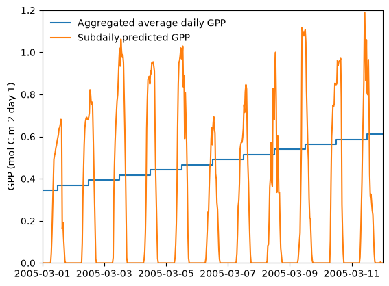
Again, to show the internal calculations, the plot below shows the predicted GPP at half hourly intervals and then the aggregated average daily assimilation used to predict LAI.
plt.step(
    phenology_fortnightly_zhou.datetimes + np.timedelta64(12, "h"),
    phenology_fortnightly_zhou.daily_potential_assimilation,
    label="Aggregated average daily GPP",
)
plt.plot(
    acclim_model.datetimes,
    subdaily_pmodel.gpp * subdaily_pmodel.gpp_conversion_factor,
    label="Subdaily predicted GPP",
)
plt.ylabel("GPP (mol C m-2 day-1)")
plt.xlim(np.datetime64("2005-03-01"), np.datetime64("2005-03-12"))
plt.ylim(0, 1.2)
_ = plt.legend(frameon=False)