Photosynthetic environment

Run this notebook

• Read the guide on setting up your computer to run Jupyter notebooks

• Download this notebook as a Jupyter notebook.

The P Model is a model of carbon capture and water use by plants. There are six core forcing variables that define the photosynthetic environment of the plant:

• the temperature (tc, °C),

• the vapor pressure deficit (vpd, Pa),

• the atmospheric \(\ce{CO2}\) concentration (co2, ppm), and

• the atmospheric pressure (patm, Pa),

• the fraction of absorbed photosynthetically active radiation (\(f_{APAR}\), fapar, unitless), and

• the photosynthetic photon flux density (PPFD, ppfd, µmol m-2 s-1)

Those forcing variables are then used to calculate further variables that capture the photosynthetic environment of a leaf. These are:

1. the photorespiratory compensation point (\(\Gamma^*\), Pascals),

2. the Michaelis-Menten coefficient for photosynthesis (\(K_{mm}\), Pascals),

3. the relative viscosity of water, given a standard at 25°C (\(\eta^*\), unitless),

4. the partial pressure of \(\ce{CO2}\) in ambient air (\(c_a\), Pascals), and

5. the absorbed irradiance (\(I_{abs}\), µmol m-2 s-1)

The descriptions below show the typical ranges of these values under common environmental inputs along with links to the more detailed documentation of the key functions.

Show code cell source

Hide code cell source

# This code loads required packages and then creates a representative range of
# values of the core variables to use in function plots.
#
# Note that the ranges are created (`_1d`) but are also cast to two dimensional
# arrays of repeating values (`_2d`) to generate response surfaces for functions
# with multiple inputs.

from matplotlib import pyplot
import numpy as np
from pyrealm.constants import CoreConst
from pyrealm.core.water import calculate_viscosity_h2o
from pyrealm.pmodel import calculate_gammastar, calculate_kmm, calculate_co2_to_ca

%matplotlib inline

# Get the default set of core constants
const = CoreConst()

# Set the resolution of examples
n_pts = 101

# Create a range of representative values for key inputs.
tc_1d = np.linspace(0, 50, n_pts)
tk_1d = tc_1d + const.k_CtoK
patm_1d = np.linspace(60000, 106000, n_pts)  # ~ tropical tree line
co2_1d = np.linspace(200, 500, n_pts)

# Broadcast the range into arrays with repeated values.
tc_2d = np.broadcast_to(tc_1d, (n_pts, n_pts))
tk_2d = np.broadcast_to(tk_1d, (n_pts, n_pts))
patm_2d = np.broadcast_to(patm_1d, (n_pts, n_pts))
co2_2d = np.broadcast_to(co2_1d, (n_pts, n_pts))

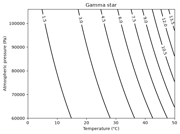
Photorespiratory compensation point (\(\Gamma^*\))

Details: pyrealm.pmodel.functions.calculate_gammastar()

The photorespiratory compensation point (\(\Gamma^*\)) varies with as a function of temperature and atmospheric pressure:

Show code cell source

Hide code cell source

# Calculate gammastar
gammastar = calculate_gammastar(tk=tk_2d, patm=patm_2d.transpose())

# Create a contour plot of gamma
fig, ax = pyplot.subplots()
CS = ax.contour(tc_1d, patm_1d, gammastar, levels=10, colors="black")
ax.clabel(CS, inline=1, fontsize=10)
ax.set_title("Gamma star")
ax.set_xlabel("Temperature (°C)")
ax.set_ylabel("Atmospheric pressure (Pa)")
pyplot.show()

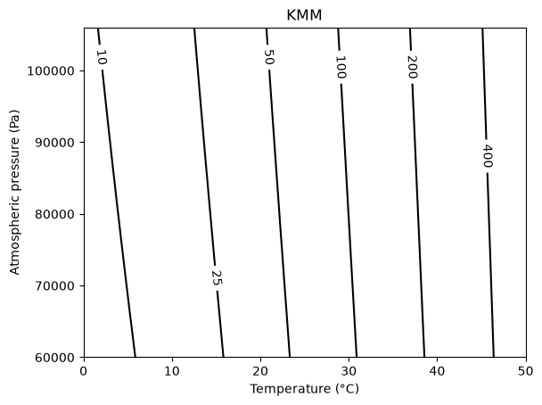
Michaelis-Menten coefficient for photosynthesis (\(K_{mm}\))

Details: pyrealm.pmodel.functions.calculate_kmm()

The Michaelis-Menten coefficient for photosynthesis (\(K_{mm}\)) also varies with temperature and atmospheric pressure:

Show code cell source

Hide code cell source

# Calculate K_mm
kmm = calculate_kmm(tk=tk_2d, patm=patm_2d.transpose())

# Contour plot of calculated values
fig, ax = pyplot.subplots()
CS = ax.contour(tc_1d, patm_1d, kmm, levels=[10, 25, 50, 100, 200, 400], colors="black")
ax.clabel(CS, inline=1, fontsize=10)
ax.set_title("KMM")
ax.set_xlabel("Temperature (°C)")
ax.set_ylabel("Atmospheric pressure (Pa)")
pyplot.show()

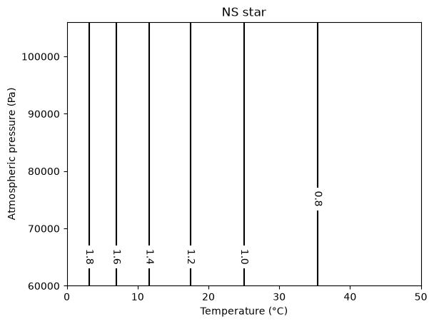
Relative viscosity of water (\(\eta^*\))

Details: calculate_density_h2o(), calculate_viscosity_h2o()

The density (\(\rho\)) and viscosity (\(\mu\)) of water both vary with temperature and atmospheric pressure. Together, these functions are used to calculate the viscosity of water relative to its viscosity at standard temperature and pressure (\(\eta^*\)).

The pyrealm package implements several alternative approaches to calculating water density and viscosity and the approaches used in calculation are controlled by the CoreConst.water_density_method and CoreConst.water_viscosity_method. The current default settings (fisher and huber) are computationally complex. You may prefer to use simpler approaches that yield very similar results but that are considerably less computationally demanding. In particular, the effects of atmospheric pressure are extremely small and are not included in most approaches.

The figure shows how \(\eta^*\) varies with temperature and pressure using the fisher and huber default settings.

Show code cell source

Hide code cell source

# Calculate the viscosity under the range of values and the standard
# temperature and pressure
viscosity = calculate_viscosity_h2o(tk=tk_2d, patm=patm_2d.transpose())
viscosity_std = calculate_viscosity_h2o(tk=const.k_To, patm=const.k_Po)

# Calculate the relative viscosity
ns_star = viscosity / viscosity_std

# Plot ns_star
fig, ax = pyplot.subplots()
CS = ax.contour(tc_1d, patm_1d, ns_star, colors="black")
ax.clabel(CS, inline=1, fontsize=10)
ax.set_title("NS star")
ax.set_xlabel("Temperature (°C)")
ax.set_ylabel("Atmospheric pressure (Pa)")
pyplot.show()

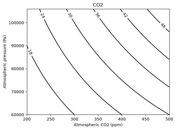
Partial pressure of \(\ce{CO2}\) (\(c_a\))

Details: pyrealm.pmodel.functions.calculate_co2_to_ca()

The partial pressure of \(\ce{CO2}\) is a function of the atmospheric concentration of \(\ce{CO2}\) in parts per million and the atmospheric pressure:

Show code cell source

Hide code cell source

# Variation in partial pressure
ca = calculate_co2_to_ca(co2_2d, patm_2d.transpose())
# Plot contour plot of values
fig, ax = pyplot.subplots()
CS = ax.contour(co2_1d, patm_1d, ca, colors="black")
ax.clabel(CS, inline=1, fontsize=10)
ax.set_title("CO2")
ax.set_xlabel("Atmospheric CO2 (ppm)")
ax.set_ylabel("Atmospheric pressure (Pa)")
pyplot.show()

Absorbed irradiation (\(I_{abs}\))

This value is simply the product of FAPAR and PPFD.