Extreme forcing values

Run this notebook

• Read the guide on setting up your computer to run Jupyter notebooks

• Download this notebook as a Jupyter notebook.

The four photosynthetic environment variables and the effect of temperature on the temperature dependence of quantum yield efficiency are all calculated directly from the input forcing variables. While the majority of those calculations behave smoothly with extreme values of temperature and atmospheric pressure, the calculation of the relative viscosity of water (\(\eta^{\ast}\)) does not handle low temperatures well.

Forcing datasets for the input to the P Model - particularly remotely sensed datasets - often contain extreme values that may lead to unexpected model predictions. This page provides an overview of the behaviour of the initial functions calculating the photosynthetic environment when given extreme inputs, to help guide when inputs should be filter or clipped to remove problem values.

Note

The PModelEnvironment implements some simple bounds checking to help guard against extreme values or errors with the units of forcing variables (see the BoundsChecker class for details).

Realistic input values

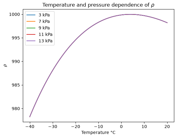
• Temperature (°C): the range of air temperatures in global datasets can easily include values as extreme as -80 °C to 50 °C. However, the water density calculation is unstable below -25°C and so PModelEnvironment will not accept values below -25°C.

• Atmospheric Pressure (Pa): at sea-level, extremes of 87000 Pa to 108400 Pa have been observed but with elevation can fall much lower, down to ~34000 Pa at the summit of Mt Everest.

• Vapour Pressure Deficit (Pa): values between extremes of 0 and 10000 Pa are realistic but some datasets may contain negative values of VPD. The problem here is that VPD is included in a square root term, which results in missing data. You should explicitly clip negative VPD values to zero or set them to np.nan.

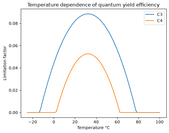
Temperature dependence of quantum yield efficiency

The quadratic equations describing the temperature dependence of quantum yield efficiency are automatically clipped to convert negative values to zero. With the default constant settings, the roots of these quadratics are:

• C4: \(-0.064 + 0.03 \cdot x - 0.000464 \cdot x^2\) has roots at 2.21 °C and 62.4 °C

• C3: \(0.352 + 0.022 \cdot x - 0.00034 \cdot x^2\) has roots at -13.3 °C and 78.0 °C

Note that the default values for C3 photosynthesis give non-zero values below 0°C.

Show code cell source

Hide code cell source

from matplotlib import pyplot
import numpy as np
from pyrealm.core.water import calculate_density_h2o
from pyrealm.constants import CoreConst
from pyrealm.pmodel import calculate_gammastar, calculate_kmm, PModelEnvironment
from pyrealm.pmodel.quantum_yield import QuantumYieldTemperature


# Set the resolution of examples
n_pts = 101

# Create environment containing a range of representative values for temperature. No
# estimation of GPP needed so fapar and ppfd set to unity
env = PModelEnvironment(
    tc=np.linspace(-25, 100, n_pts), patm=101325, vpd=820, co2=400, fapar=1, ppfd=1
)

# Calculate temperature dependence of quantum yield efficiency
fkphio_c3 = QuantumYieldTemperature(env, use_c4=False)
fkphio_c4 = QuantumYieldTemperature(env, use_c4=True)

# Create a line plot of ftemp kphio
pyplot.plot(env.tc, fkphio_c3.kphio, label="C3")
pyplot.plot(env.tc, fkphio_c4.kphio, label="C4")

pyplot.title("Temperature dependence of quantum yield efficiency")
pyplot.xlabel("Temperature °C")
pyplot.ylabel("Limitation factor")
pyplot.legend()
pyplot.show()

/home/docs/checkouts/readthedocs.org/user_builds/pyrealm/checkouts/latest/pyrealm/core/bounds.py:171: UserWarning: Variable 'tc' (°C) contains values outside the expected range (-25,80). Check units?
  warn(

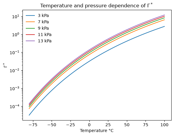
Photorespiratory compensation point (\(\Gamma^*\))

The photorespiratory compensation point (\(\Gamma^*\)) varies with as a function of temperature and atmospheric pressure, and behaves smoothly with extreme inputs. Note that again, \(\Gamma^*\) has non-zero values for sub-zero temperatures.

Show code cell source

Hide code cell source

# Calculate gammastar at different temperatures
core_const = CoreConst()
tc_1d = np.linspace(-80, 100, n_pts)
tk_1d = tc_1d + core_const.k_CtoK

# Create a contour plot of gamma
fig, ax = pyplot.subplots(1, 1)

for patm in [3, 7, 9, 11, 13]:
    pyplot.plot(
        tc_1d, calculate_gammastar(tk=tk_1d, patm=patm * 1000), label=f"{patm} kPa"
    )

ax.set_title("Temperature and pressure dependence of $\Gamma^*$")
ax.set_xlabel("Temperature °C")
ax.set_ylabel("$\Gamma^*$")
ax.set_yscale("log")
ax.legend(frameon=False)
pyplot.show()

<>:14: SyntaxWarning: invalid escape sequence '\G'
<>:16: SyntaxWarning: invalid escape sequence '\G'
<>:14: SyntaxWarning: invalid escape sequence '\G'
<>:16: SyntaxWarning: invalid escape sequence '\G'
/tmp/ipykernel_1421/3180757199.py:14: SyntaxWarning: invalid escape sequence '\G'
  ax.set_title("Temperature and pressure dependence of $\Gamma^*$")
/tmp/ipykernel_1421/3180757199.py:16: SyntaxWarning: invalid escape sequence '\G'
  ax.set_ylabel("$\Gamma^*$")

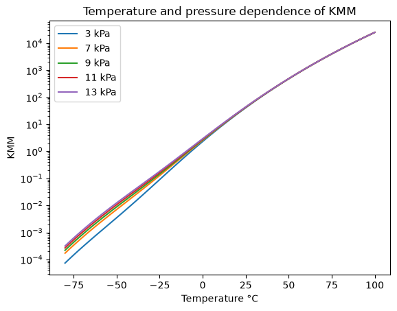
Michaelis-Menten coefficient for photosynthesis (\(K_{mm}\))

The Michaelis-Menten coefficient for photosynthesis (\(K_{mm}\)) also varies with temperature and atmospheric pressure and again behaves smoothly with extreme values.

Show code cell source

Hide code cell source

fig, ax = pyplot.subplots(1, 1)

# Calculate K_mm
for patm in [3, 7, 9, 11, 13]:
    ax.plot(tc_1d, calculate_kmm(tk=tk_1d, patm=patm * 1000), label=f"{patm} kPa")

# Create a contour plot of gamma
ax.set_title("Temperature and pressure dependence of KMM")
ax.set_xlabel("Temperature °C")
ax.set_ylabel("KMM")
ax.set_yscale("log")
ax.legend()
pyplot.show()

Relative viscosity of water (\(\eta^*\))

The density (\(\rho\)) and viscosity (\(\mu\)) of water both vary with temperature and atmospheric pressure. Looking at the density of water, there is a serious numerical issue with low temperatures arising from the equations for the density of water.

Show code cell source

Hide code cell source

fig, ax = pyplot.subplots(1, 1)

# Calculate rho
for patm in [3, 7, 9, 11, 13]:
    ax.plot(
        tc_1d,
        calculate_density_h2o(tc_1d, patm * 1000, safe=False),
        label=f"{patm} kPa",
    )

# Create a contour plot of gamma
ax.set_title(r"Temperature and pressure dependence of $\rho$")
ax.set_xlabel("Temperature °C")
ax.set_ylabel(r"$\rho$")
ax.set_yscale("log")
ax.legend()
pyplot.show()

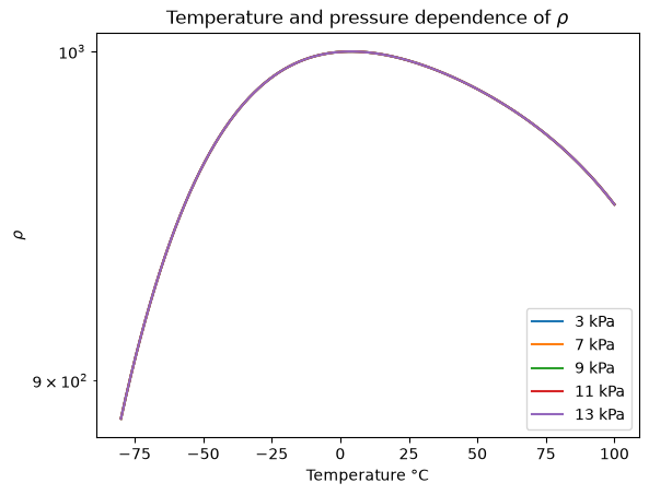
Zooming in, the behaviour of this function is not reliable at extreme low temperatures leading to unstable estimates of \(\eta^*\) and the P Model cannot be used to make predictions below -25°C.

Show code cell source

Hide code cell source

fig, ax = pyplot.subplots(1, 1)

tc_1d = np.linspace(-40, 20, n_pts)

# Calculate K_mm
for patm in [3, 7, 9, 11, 13]:
    ax.plot(
        tc_1d,
        calculate_density_h2o(tc_1d, patm * 1000, safe=False),
        label=f"{patm} kPa",
    )

# Create a contour plot of gamma
ax.set_title(r"Temperature and pressure dependence of $\rho$")
ax.set_xlabel("Temperature °C")
ax.set_ylabel(r"$\rho$")
# ax.set_yscale('log')
ax.legend()
pyplot.show()