P Model predictions

Run this notebook

• Read the guide on setting up your computer to run Jupyter notebooks

• Download this notebook as a Jupyter notebook.

Show code cell source

Hide code cell source

from itertools import product
from pyrealm.pmodel.pmodel import PModel
from pyrealm.pmodel.pmodel_environment import PModelEnvironment
import numpy as np
import matplotlib.pyplot as plt
from matplotlib.lines import Line2D

# Create inputs for a temperature curve at:
# - two atmospheric pressures
# - two CO2 concentrations
# - two VPD values

n_pts = 1001

tc_1d = np.linspace(-10, 60, n_pts)
patm_1d = np.array([101325, 80000])
vpd_1d = np.array([500, 2000])
co2_1d = np.array([280, 410])

tc_4d, patm_4d, vpd_4d, co2_4d = np.meshgrid(tc_1d, patm_1d, vpd_1d, co2_1d)

# Calculate the photosynthetic environment including approximate
# average canopy top light conditions for dry season tropical forest.
# https://doi.org/10.2307/2260066
pmodel_env = PModelEnvironment(
    tc=tc_4d, patm=patm_4d, vpd=vpd_4d, co2=co2_4d, fapar=0.91, ppfd=600
)

# Run the P Models
pmodel_c3 = PModel(pmodel_env)
pmodel_c4 = PModel(pmodel_env, method_optchi="c4")


# Create line plots of optimal chi

# Create a list of combinations and line formats
# (line col: PATM, style: CO2, marker used for VPD)

idx_vals = {
    "vpd": zip([0, 1], vpd_1d),
    "patm": zip([0, 1], patm_1d),
    "co2": zip([0, 1], co2_1d),
}

idx_combos = list(product(*idx_vals.values()))
line_formats = ["r-", "r--", "b-", "b--"] * 2


def plot_fun(estvar, estvarlab):
    """Helper function to plot an estimated variable

    Args:
        estvar: String naming variable to be plotted
        estvarlab: String to be used in axis labels
    """

    # Create side by side subplots
    fig, (ax1, ax2) = plt.subplots(1, 2, figsize=(12, 5), sharey=True, sharex=True)

    # Loop over the envnt combinations for c3 and c4 models
    for this_mod, this_axs in zip((pmodel_c3, pmodel_c4), (ax1, ax2)):

        for ((vdx, vvl), (pdx, pvl), (cdx, cvl)), lfmt in zip(idx_combos, line_formats):

            mrkr = "o" if vvl == 500 else "^"
            plotvar = getattr(this_mod, estvar)

            this_axs.plot(tc_1d, plotvar[pdx, :, vdx, cdx], lfmt)
            max_idx = np.nanargmax(plotvar[pdx, :, vdx, cdx])
            this_axs.scatter(
                tc_1d[max_idx],
                plotvar[pdx, :, vdx, cdx][max_idx],
                marker=mrkr,
                s=60,
                c="none",
                edgecolor="black",
            )

        # Set axis labels
        this_axs.set_xlabel("Temperature °C")
        this_axs.set_ylabel(f"Estimated {estvarlab}")

    ax1.set_title(f"C3 variation in estimated {estvarlab}")
    ax2.set_title(f"C4 variation in {estvarlab}")

    plt.show()

/home/docs/checkouts/readthedocs.org/user_builds/pyrealm/checkouts/latest/pyrealm/pmodel/pmodel.py:481: UserWarning: 
    Pyrealm 2.0.0 uses a new default for the quantum yield of photosynthesis (phi0=1/8).
    You may need to change settings to duplicate results from pyrealm 1.0.0.
            
  warn(

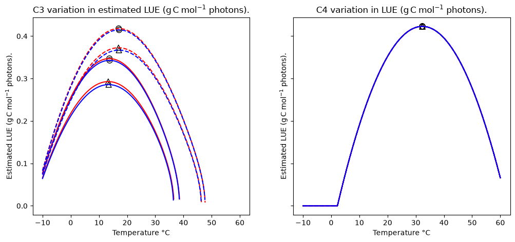
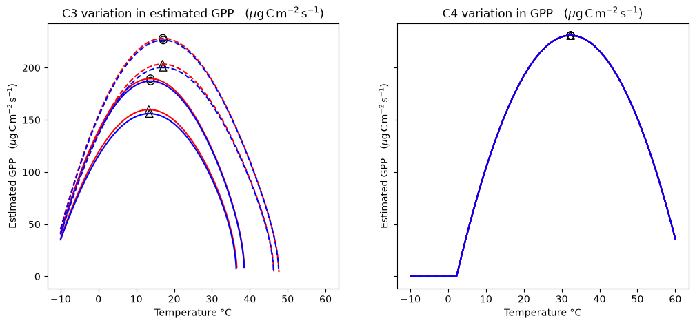
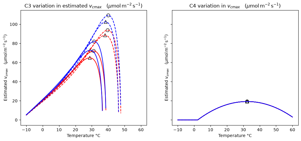
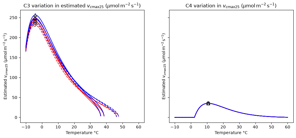
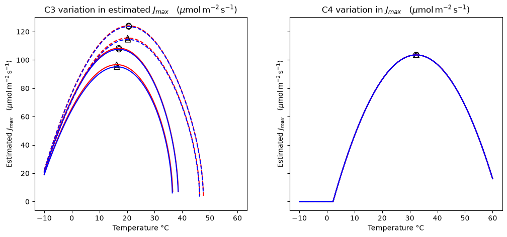
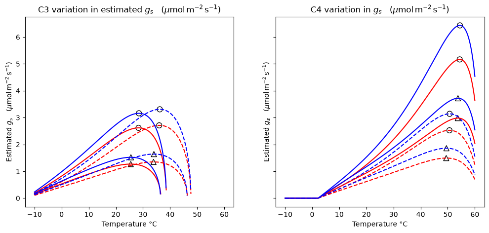
This page shows how the main output variables from the P Model vary under differing environmental conditions. The paired plots below show how C3 and C4 plants respond under a range of temperatures (-10°C to 60°C) and then pairs of values for the other environmental variables:

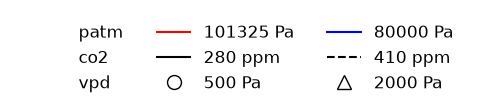
• Atmospheric pressure: 101325 Pa and 80000 Pa

• Vapour pressure deficit: 500 Pa and 2000 Pa

• \(\ce{CO2}\) concentration: 280 ppm and 410 ppm.

For the plots below, productivity has been estimated using a representative irradiance values at the top of a tropical rainforest canopy:

• \(f_{APAR}\): 0.91 (unitless)

• PPFD: 600 µmol m-2 s-1

Warning

The estimated PPFD must be expressed as µmol m-2 s-1.

Estimates of PPFD sometimes use different temporal or spatial scales - for example daily moles of photons per hectare. Although GPP can also be expressed with different units, many other predictions of the P Model (\(J_{max}\), \(V_{cmax}\), \(g_s\) and \(r_d\)) must be expressed as µmol m-2 s-1 and so this standard unit must also be used for PPFD.

All of the pairwise plots share the same legend:

Show code cell source

Hide code cell source

fig, ax = plt.subplots(1, 1, figsize=(6, 1.2))

# create a legend showing the combinations
blnk = Line2D([], [], color="none")
rd = Line2D([], [], linestyle="-", color="r")
bl = Line2D([], [], linestyle="-", color="b")
sld = Line2D([], [], linestyle="-", color="k")
dsh = Line2D([], [], linestyle="--", color="k")
circ = Line2D(
    [],
    [],
    marker="o",
    linestyle="",
    markersize=10,
    markeredgecolor="k",
    markerfacecolor="none",
)
trng = Line2D(
    [],
    [],
    marker="^",
    linestyle="",
    markersize=10,
    markeredgecolor="k",
    markerfacecolor="none",
)

ax.legend(
    [blnk, blnk, blnk, rd, sld, circ, bl, dsh, trng],
    [
        "patm",
        "co2",
        "vpd",
        f"{patm_1d[0]} Pa",
        f"{co2_1d[0]} ppm",
        f"{vpd_1d[0]} Pa",
        f"{patm_1d[1]} Pa",
        f"{co2_1d[1]} ppm",
        f"{vpd_1d[1]} Pa",
    ],
    ncol=3,
    loc="upper center",
    frameon=False,
    prop={"size": 12},
)

ax.axis("off")

plt.show()

Efficiency outputs

Light use efficiency (lue, LUE)

Light use efficiency measures conversion efficiency of moles of absorbed irradiance into grams of Carbon (\(\mathrm{g\,C}\; \mathrm{mol}^{-1}\) photons).

Show code cell source

Hide code cell source

plot_fun("lue", r"LUE ($\mathrm{g\,C}\; \mathrm{mol}^{-1}$ photons).")

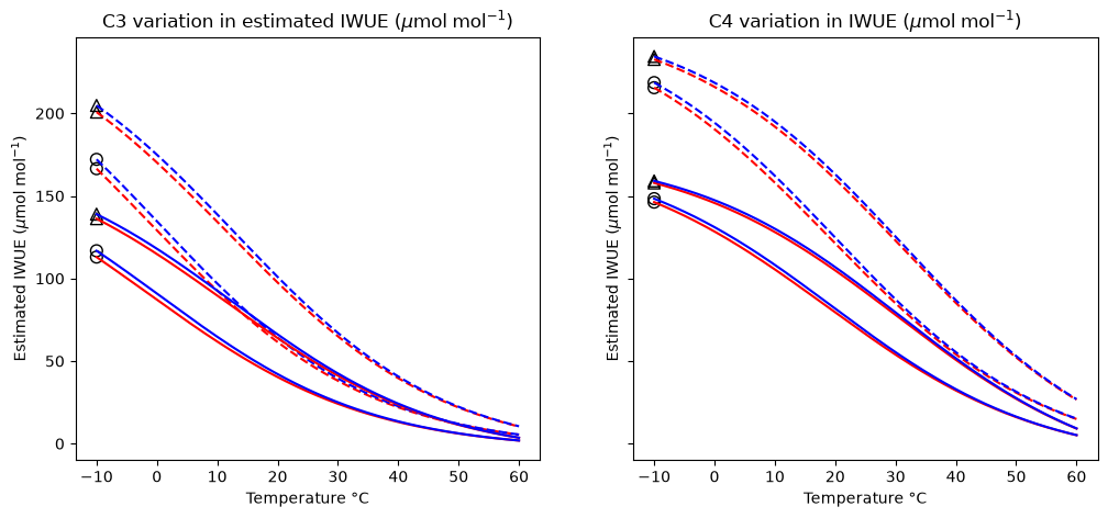
Intrinsic water use efficiency (iwue, IWUE)

The intrinsic water-use efficiency is ratio of net photosynthetic CO2 assimilation to stomatal conductance, and captures the cost of assimilation per unit of water, in units of \(\mu\mathrm{mol}\;\mathrm{mol}^{-1}\).

Show code cell source

Hide code cell source

plot_fun("iwue", r"IWUE ($\mu\mathrm{mol}\;\mathrm{mol}^{-1}$)")

Productivity outputs

The remaining key outputs are measures of photosynthetic productivity, such as GPP, which are calculated using the provided estimates of PPFD and FAPAR and the resulting absorbed irradiance (\(I_{abs}\)).

The productivity variables and their units are:

• Gross primary productivity (gpp, \(\mu\text{gC}\,\mathrm{m}^{-2}\,\text{s}^{-1}\))

• Maximum rate of carboxylation (vcmax, \(\mu\text{mol}\,\mathrm{m}^{-2}\,\text{s}^{-1}\))

• Maximum rate of carboxylation at standard temperature (vcmax25, \(\mu\text{mol}\,\mathrm{m}^{-2}\,\text{s}^{-1}\))

• Maximum rate of electron transport. (jmax, \(\mu\text{mol}\,\mathrm{m}^{-2}\,\text{s}^{-1}\))

• Stomatal conductance (gs, \(\mu\text{mol}\,\mathrm{m}^{-2}\,\text{s}^{-1}\))

Gross primary productivity (gpp, GPP)

Show code cell source

Hide code cell source

plot_fun("gpp", r"GPP   ($\mu\mathrm{g\,C}\,\mathrm{m}^{-2}\,\mathrm{s}^{-1}$)")

Maximum rate of carboxylation (vcmax)

Show code cell source

Hide code cell source

plot_fun("vcmax", r"$v_{cmax}$   ($\mu\mathrm{mol}\,\mathrm{m}^{-2}\,\mathrm{s}^{-1}$)")

Maximum rate of carboxylation at standard temperature (vcmax25)

Show code cell source

Hide code cell source

plot_fun(
    "vcmax25", r"$v_{cmax25}$ ($\mu\mathrm{mol}\,\mathrm{m}^{-2}\,\mathrm{s}^{-1}$)"
)

Maximum rate of electron transport. (jmax)

Show code cell source

Hide code cell source

plot_fun("jmax", r"$J_{max}$   ($\mu\mathrm{mol}\,\mathrm{m}^{-2}\,\mathrm{s}^{-1}$)")

Stomatal conductance (gs, \(g_s\))

Stomatal conductance is estimated using the difference between ambient and optimal internal leaf \(\ce{CO2}\) concentration. When vapour pressure deficit is zero, the difference between \(c_a\) and \(c_i\) will tend to zero, which leads to numerical instability in estimates of \(g_s\), which will be set as undefined (np.nan) when VPD is zero or when \(c_a - c_i = 0\).

Show code cell source

Hide code cell source

plot_fun("gs", r"$g_s$   ($\mu\mathrm{mol}\,\mathrm{m}^{-2}\,\mathrm{s}^{-1}$)")

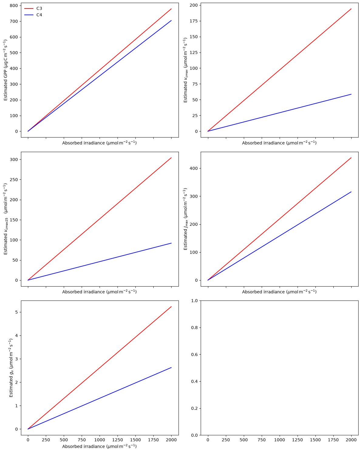
Scaling with absorbed irradiance

All of the six productivity variables scale linearly with absorbed irradiance. The plots below show how each variable changes, for a constant environment with tc of 20°C, patm of 101325 Pa, vpd of 1000 Pa and \(\ce{CO2}\) of 400 ppm, when absorbed irradiance changes from 0 to 2000 \(\mu\text{mol}\,\mathrm{m}^{-2}\,\text{s}^{-1}\).

Show code cell source

Hide code cell source

# Calculate the photosynthetic environment
ppfd_vals = np.arange(2000)
pmodel_env = PModelEnvironment(
    tc=20, patm=101325, vpd=1000, co2=400, fapar=1, ppfd=ppfd_vals
)

# Run the P Models
pmodel_c3 = PModel(pmodel_env)
pmodel_c4 = PModel(pmodel_env, method_optchi="c4")


def plot_iabs(ax, estvar, estvarlab):
    """Helper function to plot an estimated variable

    Args:
        estvar: String naming variable to be plotted
        estvarlab: String to be used in axis labels
    """

    # Loop over the envnt combinations for c3 and c4 models
    for this_mod, lfmt in zip((pmodel_c3, pmodel_c4), ("r-", "b-")):

        plotvar = getattr(this_mod, estvar)
        ax.plot(ppfd_vals, plotvar, lfmt)

    # Set axis labels
    ax.set_xlabel(
        r"Absorbed irradiance ($\mu\mathrm{mol}\,\mathrm{m}^{-2}\,\mathrm{s}^{-1}$)"
    )
    ax.set_ylabel(f"Estimated {estvarlab}")


fig, axs = plt.subplots(3, 2, figsize=(12, 15), sharex=True)

plot_iabs(
    axs[0, 0], "gpp", r"GPP ($\mu\mathrm{g\,C}\,\mathrm{m}^{-2}\,\mathrm{s}^{-1}$)"
)

plot_iabs(
    axs[0, 1],
    "vcmax",
    r"$v_{cmax}$ ($\mu\mathrm{mol}\,\mathrm{m}^{-2}\,\mathrm{s}^{-1}$)",
)
plot_iabs(
    axs[1, 0],
    "vcmax25",
    r"$v_{cmax25}$   ($\mu\mathrm{mol}\,\mathrm{m}^{-2}\,\mathrm{s}^{-1}$)",
)
plot_iabs(
    axs[1, 1],
    "jmax",
    r"$J_{max}$ ($\mu\mathrm{mol}\,\mathrm{m}^{-2}\,\mathrm{s}^{-1}$)",
)
plot_iabs(
    axs[2, 0], "gs", r"$g_s$ ($\mu\mathrm{mol}\,\mathrm{m}^{-2}\,\mathrm{s}^{-1}$)"
)

axs[0, 0].legend(
    [
        Line2D([], [], linestyle="-", color="r"),
        Line2D([], [], linestyle="-", color="b"),
    ],
    ["C3", "C4"],
    loc="upper left",
    frameon=False,
)

fig.tight_layout()
plt.show()