Subdaily P Model calculations

Run this notebook

• Read the guide on setting up your computer to run Jupyter notebooks

• Download this notebook as a Jupyter notebook.

The code below works through the separate calculations used to include the acclimation of slow responses into the predictions of the P Model. The code separates out individual steps used in the estimation process in order to show intermediate results and provides an “exploded diagram” of the model. In practice, these calculations are handled internally by the model fitting in pyrealm, as shown in the worked example.

Show code cell source

Hide code cell source

from importlib import resources

from matplotlib import pyplot as plt
import matplotlib.dates as mdates
import numpy as np
import pandas

from pyrealm.pmodel import (
    PModel,
    SubdailyPModel,
    PModelEnvironment,
    AcclimationModel,
    calculate_simple_arrhenius_factor,
)
from pyrealm.pmodel.optimal_chi import OptimalChiPrentice14
from pyrealm.pmodel.quantum_yield import QuantumYieldTemperature
from pyrealm.pmodel.arrhenius import SimpleArrhenius

Example dataset

The code below uses half hourly data from 2014 for the BE-Vie FluxNET site, which was also used as a demonstration in Mengoli et al. (2022).

data_path = resources.files("pyrealm_build_data.subdaily") / "subdaily_BE_Vie_2014.csv"

data = pandas.read_csv(str(data_path))

# Extract the key half hourly timestep variables as numpy arrays
temp_subdaily = data["ta"].to_numpy()
vpd_subdaily = data["vpd"].to_numpy()
co2_subdaily = data["co2"].to_numpy()
patm_subdaily = data["patm"].to_numpy()
ppfd_subdaily = data["ppfd"].to_numpy()
fapar_subdaily = data["fapar"].to_numpy()
datetime_subdaily = pandas.to_datetime(data["time"]).to_numpy()

Photosynthetic environment

This dataset can then be used to calculate the photosynthetic environment at the subdaily timescale. The code below also estimates GPP under the standard P Model with no slow responses for comparison.

# Calculate the photosynthetic environment
subdaily_env = PModelEnvironment(
    tc=temp_subdaily,
    vpd=vpd_subdaily,
    co2=co2_subdaily,
    patm=patm_subdaily,
    ppfd=ppfd_subdaily,
    fapar=fapar_subdaily,
)

# Fit the standard P Model
pmodel_standard = PModel(subdaily_env)
pmodel_standard.summarize()

PModel(shape=(17520,), method_optchi=prentice14, method_arrhenius=simple, method_jmaxlim=wang17, method_kphio=temperature)
Attr       Mean    Min     Max    NaN  Units
-------  ------  -----  ------  -----  ------------
lue        0.4    0.14    0.48      0  g C mol-1
iwue      36.48  -0     108.75      0  µmol mol-1
gpp       65.08   0     625.02    176  µg C m-2 s-1
vcmax     12.99   0     187.94    176  µmol m-2 s-1
vcmax25   33.35   0     376.83    176  µmol m-2 s-1
gs         0.8    0      13.04   7500  µmol m-2 s-1
jmax      34.76   0     344.55    176  µmol m-2 s-1
jmax25    68.61   0     776.56    176  µmol m-2 s-1

/home/docs/checkouts/readthedocs.org/user_builds/pyrealm/checkouts/latest/pyrealm/pmodel/pmodel.py:481: UserWarning: 
    Pyrealm 2.0.0 uses a new default for the quantum yield of photosynthesis (phi0=1/8).
    You may need to change settings to duplicate results from pyrealm 1.0.0.
            
  warn(

The code below then fits a P Model including slow responses, which requires the definition of a daily acclimation window, identifying the daily conditions that will lead to optimal overall productivity. While acclimating to average daytime environment might give better overall light use efficiency across the day, productivity is optimised by acclimating to the conditions when PPFD is high.

A decision needs to be made about when those conditions occur during the day and how best to sample those conditions. Typically those might be the observed environmental conditions at the observation closest to noon, or the mean environmental conditions in a window around noon.

# Create the acclimation model
acclim_model = AcclimationModel(datetime_subdaily, allow_holdover=True, alpha=1 / 15)

# Set the acclimation window as the values within a one hour window centred on noon
acclim_model.set_window(
    window_center=np.timedelta64(12, "h"),
    half_width=np.timedelta64(30, "m"),
)

# Fit the Subdaily P Model
pmodel_subdaily = SubdailyPModel(
    env=subdaily_env,
    acclim_model=acclim_model,
)

Show code cell source

Hide code cell source

idx = np.arange(48 * 120, 48 * 130)
plt.figure(figsize=(10, 4))
plt.plot(datetime_subdaily[idx], pmodel_standard.gpp[idx], label="Instantaneous model")
plt.plot(datetime_subdaily[idx], pmodel_subdaily.gpp[idx], "r-", label="Slow responses")
plt.ylabel("GPP (gc m-2 s-1)")
plt.legend(frameon=False)
plt.show()

Calculation of GPP using fast and slow responses

The SubdailyPModel implements the calculations used to estimate GPP using slow responses, but the details of these calculations are shown below.

Optimal responses during the acclimation window

The daily average conditions during the acclimation window can be sampled and used as inputs to the standard P Model to calculate the optimal behaviour of plants under those conditions.

# Get the daily acclimation conditions for the forcing variables
temp_acclim = acclim_model.get_daily_means(temp_subdaily)
co2_acclim = acclim_model.get_daily_means(co2_subdaily)
vpd_acclim = acclim_model.get_daily_means(vpd_subdaily)
patm_acclim = acclim_model.get_daily_means(patm_subdaily)
ppfd_acclim = acclim_model.get_daily_means(ppfd_subdaily)
fapar_acclim = acclim_model.get_daily_means(fapar_subdaily)

# Fit the P Model to the acclimation conditions
daily_acclim_env = PModelEnvironment(
    tc=temp_acclim,
    vpd=vpd_acclim,
    co2=co2_acclim,
    patm=patm_acclim,
    fapar=fapar_acclim,
    ppfd=ppfd_acclim,
)

pmodel_acclim = PModel(daily_acclim_env)

Slow responses of \(\xi\), \(J_{max25}\) and \(V_{cmax25}\)

Rather than being able to instantaneously adopt optimal values, the \(\xi\), \(J_{max25}\) and \(V_{cmax25}\) parameters are assumed to acclimate towards optimal values with a lagged response using a memory effect.

Calculation of \(J_{max}\) and \(V_{cmax}\) at standard temperature

The daily optimal acclimation values are obviously calculated under a range of temperatures so \(J_{max}\) and \(V_{cmax}\) must first be standardised to expected values at 25°C. This is achieved calculating an Arrhenius scaling factor for the temperature of the observation relative to the standard temperature, given the activation energy of the enzymes.

pmodel_const = pmodel_subdaily.env.pmodel_const
core_const = pmodel_subdaily.env.core_const

tk_acclim = temp_acclim + core_const.k_CtoK
tk_ref = pmodel_const.tk_ref

arrh_daily = SimpleArrhenius(env=daily_acclim_env)

vcmax25_acclim = pmodel_acclim.vcmax / arrh_daily.calculate_arrhenius_factor(
    pmodel_const.arrhenius_vcmax
)
jmax25_acclim = pmodel_acclim.jmax / arrh_daily.calculate_arrhenius_factor(
    pmodel_const.arrhenius_jmax
)

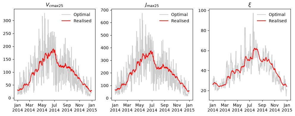
Calculation of realised values

The memory effect can now be applied to the three parameters with slow responses to calculate realised values, here using the default 15 day window.

# Calculation of memory effect in xi, vcmax25 and jmax25
xi_real = acclim_model.apply_acclimation(pmodel_acclim.optchi.xi)
vcmax25_real = acclim_model.apply_acclimation(vcmax25_acclim)
jmax25_real = acclim_model.apply_acclimation(jmax25_acclim)

The plots below show the instantaneously acclimated values for \(J_{max25}\), \(V_{cmax25}\) and \(\xi\) in grey along with the realised slow responses, after application of the memory effect.

Show code cell source

Hide code cell source

fig, axes = plt.subplots(1, 3, figsize=(12, 4))

for ax, inst, mem, title in zip(
    axes,
    (vcmax25_acclim, jmax25_acclim, pmodel_acclim.optchi.xi),
    (vcmax25_real, jmax25_real, xi_real),
    (r"$V_{cmax25}$", r"$J_{max25}$", r"$\xi$"),
):

    ax.plot(acclim_model.observation_dates, inst, "0.8", label="Optimal")
    ax.plot(acclim_model.observation_dates, mem, "r-", label="Realised")
    ax.set_title(title)
    ax.legend(frameon=False)

    myFmt = mdates.DateFormatter("%b\n%Y")
    ax.xaxis.set_major_formatter(myFmt)

Subdaily model including fast and slow responses

The last stage is to recalculate P model predictions on the subdaily timescale using the realised slow responses for \(\xi\), \(J_{max25}\) and \(V_{cmax25}\).

Calculation of fast responses in \(J_{max}\) and \(V_{cmax}\)

Although the maximum rates at standard temperature \(J_{max25}\) and \(V_{cmax25}\) exhibit slow responses, the values of \(J_{max}\) and \(V_{cmax}\) will respond to changes in temperature at fast scales:

• The realised daily values of \(J_{max25}\) and \(V_{cmax25}\) are interpolated from the acclimation window to the subdaily time scale.

• These values are adjusted to the actual half hourly temperatures to give the fast responses of \(J_{max}\) and \(V_{cmax}\).

# Fill the realised jmax and vcmax from subdaily to daily
vcmax25_subdaily = acclim_model.fill_daily_to_subdaily(vcmax25_real)
jmax25_subdaily = acclim_model.fill_daily_to_subdaily(jmax25_real)

# Get the Arrhenius scaler
arrh_subdaily = SimpleArrhenius(env=subdaily_env)

# Adjust to actual temperature at subdaily timescale
vcmax_subdaily = vcmax25_subdaily * arrh_subdaily.calculate_arrhenius_factor(
    coefficients=pmodel_const.arrhenius_vcmax
)
jmax_subdaily = jmax25_subdaily * arrh_subdaily.calculate_arrhenius_factor(
    coefficients=pmodel_const.arrhenius_jmax
)

Calculation of \(c_i\)

The subdaily variation in \(c_i\) can now be calculated using \(c_a\) and fast responses in \(\Gamma^\ast\) with the realised slow responses of \(\xi\). This is achieved by passing the realised values of \(\xi\) as a fixed constraint to the calculation of optimal \(\chi\), rather than calculating the instantaneously optimal values of \(\xi\) as is the case in the standard P Model.

# Interpolate xi to subdaily scale
xi_subdaily = acclim_model.fill_daily_to_subdaily(xi_real)

# Calculate the optimal chi, imposing the realised xi values
subdaily_chi = OptimalChiPrentice14(env=subdaily_env)
subdaily_chi.estimate_chi(xi_values=xi_subdaily)

# Calculate ci
ci_subdaily = subdaily_chi.ci

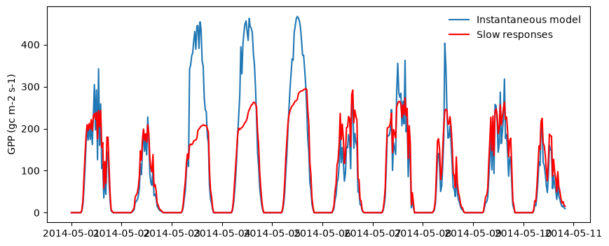
Calculation of assimilation and GPP

Predictions for \(A_j\), \(A_c\) and GPP can then now be calculated as in the standard P Model, where \(c_i\) includes the slow responses of \(\xi\) and \(V_{cmax}\) and \(J_{max}\) include the slow responses of \(V_{cmax25}\) and \(J_{max25}\) and fast responses to temperature.

# Calculate Ac
Ac_subdaily = (
    vcmax_subdaily
    * (subdaily_chi.ci - subdaily_env.gammastar)
    / (subdaily_chi.ci + subdaily_env.kmm)
)

# Calculate J and Aj
phi = QuantumYieldTemperature(env=subdaily_env)
iabs = fapar_subdaily * ppfd_subdaily

J_subdaily = (4 * phi.kphio * iabs) / np.sqrt(
    1 + ((4 * phi.kphio * iabs) / jmax_subdaily) ** 2
)

Aj_subdaily = (
    (J_subdaily / 4)
    * (subdaily_chi.ci - subdaily_env.gammastar)
    / (subdaily_chi.ci + 2 * subdaily_env.gammastar)
)

# Calculate GPP and convert from micromols to micrograms
GPP_subdaily = (
    np.minimum(Ac_subdaily, Aj_subdaily) * pmodel_subdaily.env.core_const.k_c_molmass
)

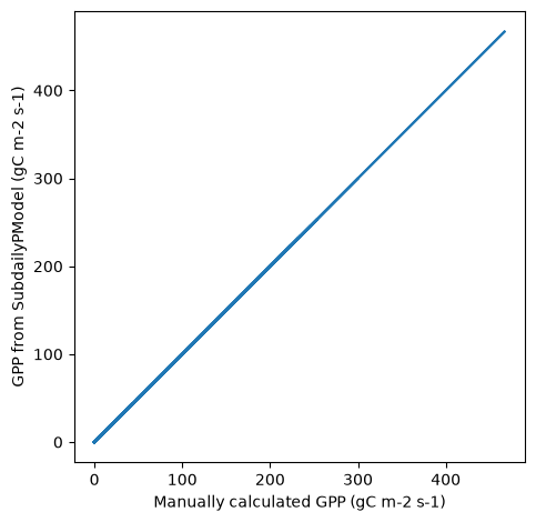
# Compare to the SubdailyPModel outputs
fig, ax = plt.subplots()
ax.plot(GPP_subdaily, pmodel_subdaily.gpp)
ax.set_xlabel("Manually calculated GPP (gC m-2 s-1)")
ax.set_ylabel("GPP from SubdailyPModel (gC m-2 s-1)")
ax.set_aspect("equal")
plt.tight_layout()