Estimating maximum annual \(f_{APAR}\)
Run this notebook
Read the guide on setting up your computer to run Jupyter notebooks
Download
this notebookas a Jupyter notebook.
The FaparLimitation class calculates
annual maximum values for both \(f_{APAR}\) and leaf area index (\(L\)). Two alternative
approaches are available via the method argument:
the option
method=caiimplements the approach of Cai et al. (2025), andthe option
method=zhuimplements the approach of Zhu et al. (2026).
In both cases, the maximum annual fAPAR is limited by the ability of plants to assimilate carbon for constructing leaves. This can be limited either by the availability of light energy (\(f_{APAR_{c}}\)) or by the availability of water (\(f_{APAR_{w}}\)). The equations are:
Five of the terms above are annual estimates for a site of:
The ambient CO2 partial pressure during the growing season (\(c_a\), Pa).
The annual mean vapour pressure deficit during the growing season (\(D\), Pa)
The annual total precipitation (\(P\), \(\text{mol m}^{-2} \text{year}^{-1}\))
The annual mean ratio of ambient to leaf CO2 partial during the growing season (\(\chi\), Pa)
The annual total potential GPP expressed in moles of Carbon (\(A_0\), \(\text{mol C m}^{-2} \text{year}^{-1}\)).
The remaining variables are:
the light extinction coefficient of leaves (\(k\)),
the growth and maintenance costs of leaves (\(z\)), and
the ratio of annual total transpiration to annual total precipitation (\(f_0\)).
The methods differ in the values used for \(z\) and \(f_0\) and in the calculation of annual maximum fAPAR from the water limited and energy limited terms.
The option
method=caiuses a fixed value for \(z\) but calculates \(f_0\) as a function of the site-specific long term aridity index expressed as PET/P (seeFaparLimitationMethodCai.set_z_and_f0for details). The maximum annual fAPAR for a site is then simply the minimum of the energy and water limited terms for that site.Using this method requires that users provide those site specific aridity values in addition to the other variables required for calculation.
The option
method=zhuuses fixed values for both \(z\) and \(f_0\), but the maximum annual fAPAR is a function of the energy limited and water limited terms, following the model of the Budyko curve (Roderick and Farquhar, 2011) (seeFaparLimitationMethodZhu.calculate_maximum_faparfor details).
In both cases, best fit global values of \(z\) and \(f_0\) (or parameters of the function
for \(f_0\)) were estimated from satellite derived fAPAR and environmental data. These
values are defined in the
PhenologyConst constants object, which can
be updated with user defined values.
From the maximum annual fAPAR, the maximum leaf area index (\(L_{max}\)) is approximated using Beer’s law:
Example calculations
The examples below uses a time series of half hourly data from the DE_Gri
Fluxnet site from 2004 to 2014 that
has been resampled to show different workflows for calculating annual maximum fAPAR.
The different workflows use some site specific scalar values, loaded in the following
code.
# Load site data
site_data_path = get_pyrealm_data("phenology/inputs/source/DE-GRI_site_data.json")

with open(site_data_path) as json_src:
    site_data = json.load(json_src)
Direct calculation from annual values
Directly calculating annual maximum fAPAR using
FaparLimitation requires you to
provide the calculated annual summary statistics given in the equations above. The
example data contains estimates of these annual values calculated from the original half
hourly FluxNET data and from a separately fitted model of assimilation.
# Load annual estimates
annual_data_path = get_pyrealm_data("phenology/inputs/fortnightly/annual_inputs.csv")
annual_data = pd.read_csv(annual_data_path)
annual_data["time"] = annual_data["year"].to_numpy().astype(str).astype("datetime64[Y]")
The plots below show the annual estimates of the required variables from the
annual_data dataset:

The code below then shows the use of the different methods available within the
FaparLimitation class to calculate
\(f_{APAR_{max}}\) and \(L_{max}\). Note that method="cai" requires additional
aridity_index data and that these should be an array providing a single climatological
estimate per site. For example, a dataset covering a 5x5 grid of sites over 20 years
would have annual data with the shape (20, 5, 5) and so the aridity data would be an
array with shape (5, 5). When there is only a single site, the site data should be a
“scalar” array of size (1,) as in the example below.
faparlim_cai = FaparLimitation(
    method="cai",
    annual_total_potential_gpp=annual_data["annual_total_A0"].to_numpy(),
    annual_mean_ca=annual_data["annual_mean_ca_in_GS"].to_numpy(),
    annual_mean_chi=annual_data["annual_mean_chi_in_GS"].to_numpy(),
    annual_mean_vpd=annual_data["annual_mean_VPD_in_GS"].to_numpy(),
    annual_total_precip=annual_data["annual_precip_molar"].to_numpy(),
    annual_growing_season_length=annual_data["N_growing_days"].to_numpy(),
    years=annual_data["time"].to_numpy().astype("datetime64[Y]"),
    aridity_index=np.array([site_data["AI_from_cruts"]]),
)

faparlim_cai.summarize()
FaparLimitation(shape=(11,))
Attr         Mean    Min    Max    NaN  Units
---------  ------  -----  -----  -----  -------
lai_max       4.7   4.37   4.93      0  -
fapar_max     0.9   0.89   0.92      0  -
/home/docs/checkouts/readthedocs.org/user_builds/pyrealm/checkouts/latest/pyrealm/core/experimental.py:72: ExperimentalFeatureWarning: 'Be aware that FaparLimitation is an experimental feature of pyrealm and the implementation and API may change within major versions.'
  warn(qualname, ExperimentalFeatureWarning)
faparlim_zhu = FaparLimitation(
    method="zhu",
    annual_total_potential_gpp=annual_data["annual_total_A0"].to_numpy(),
    annual_mean_ca=annual_data["annual_mean_ca_in_GS"].to_numpy(),
    annual_mean_chi=annual_data["annual_mean_chi_in_GS"].to_numpy(),
    annual_mean_vpd=annual_data["annual_mean_VPD_in_GS"].to_numpy(),
    annual_total_precip=annual_data["annual_precip_molar"].to_numpy(),
    annual_growing_season_length=annual_data["N_growing_days"].to_numpy(),
    years=annual_data["time"].to_numpy().astype("datetime64[Y]"),
)

faparlim_zhu.summarize()
FaparLimitation(shape=(11,))
Attr         Mean    Min    Max    NaN  Units
---------  ------  -----  -----  -----  -------
lai_max      3.74   3.54   3.98      0  -
fapar_max    0.85   0.83   0.86      0  -
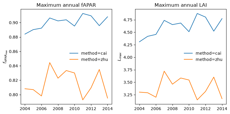
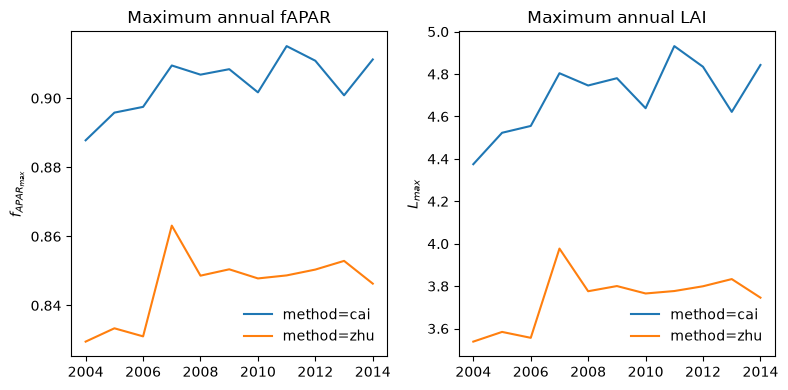
The resulting time series of annual values of \(f_{APAR_{max}}\) and \(L_{max}\) are shown below:
Calculation from a fitted PModel
Calculating annual maximum fAPAR requires the use of a P Model to provide estimates of \(A_0\) and \(\chi\) and fitting a P Model also requires data on VPD and CO2 concentration. However, a P model is typically fitted to data at faster temporal scales than the annual values required to calculate maximum fAPAR.
The standard P Model typically uses monthly to weekly observations
The subdaily P Model is fitted to observations at subdaily frequencies.
To make it easier to estimate maximum \(f_{APAR}\) the
FaparLimitation.from_pmodel
method can be used to automatically calculate the required annual summary statistics
using the dates and times of the observations used in the P Model (see the
AnnualValueCalculator class for details). The method
also handles all of unit conversion needed to estimate annual maximum fAPAR.
The method does require some additional data that is not required when fitting a P model:
growing_seasonThe calculation of \(f_{APAR_{max}}\) requires estimates of \(D, c_a\) and \(\chi\) during the growing season. The
growing_seasoninput is an array of boolean (TrueorFalse) values that indicates if each observation was during the growing season. There are different approaches for estimating the start and end of the growing season and so you need to create this variable according to the approach you want to use - it is often simply if the temperature exceeds a certain threshold.precipThe P Model does not require precipitation data, so this must be added when using
from_pmodel. You will need to compile data for the total precipitation during each observation, expressed as the total precipitation during each period of observation in moles of water per m2.datetimesDatestamps are needed to map the data in the PModel onto years to map the observations onto years and to scale per second rates from the P Model up to the annual time scale. This is only needed when using the standard P Model (see below)
The standard P Model
The example here uses fortnightly summary data for the DE_Gri dataset to fit a
standard P Model. The data provides 287 observations of fortnightly average conditions
for the site over 11 years.
# Load fortnightly data
fortnightly_data_path = get_pyrealm_data(
    "phenology/inputs/fortnightly/pmodel_inputs.csv"
)
fortnightly_data = pd.read_csv(fortnightly_data_path)
fortnightly_data["time"] = pd.to_datetime(fortnightly_data["time"])
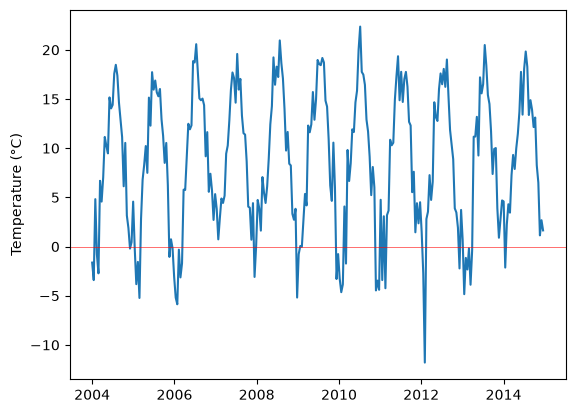
The plot below shows the time series for temperature.
That data can then be used to fit a P model for the site. Note that setting \(f_{APAR} = 1\) is required to calculate potential GPP for estimating maximum fAPAR.
pmodel_env = PModelEnvironment(
    tc=fortnightly_data["tc"].to_numpy(),
    vpd=fortnightly_data["vpd"].to_numpy(),
    patm=fortnightly_data["patm"].to_numpy(),
    co2=fortnightly_data["co2"].to_numpy(),
    ppfd=fortnightly_data["ppfd"].to_numpy(),
    fapar=np.array([1]),
)
pmodel = PModel(pmodel_env)

pmodel.summarize()
PModel(shape=(287,), method_optchi=prentice14, method_arrhenius=simple, method_jmaxlim=wang17, method_kphio=temperature)
Attr       Mean    Min     Max    NaN  Units
-------  ------  -----  ------  -----  ------------
lue        0.37   0.04    0.44      0  g C mol-1
iwue      79.52  48.98  107.97      0  µmol mol-1
gpp       97.69   5.91  234.02      0  µg C m-2 s-1
vcmax     17.61   0.57   59.11      0  µmol m-2 s-1
vcmax25   57.92   8.78  146.5       0  µmol m-2 s-1
gs         0.66   0.03    1.53      0  µmol m-2 s-1
jmax      51.38   2.76  131.58      0  µmol m-2 s-1
jmax25   117.84  17.15  292.07      0  µmol m-2 s-1
/home/docs/checkouts/readthedocs.org/user_builds/pyrealm/checkouts/latest/pyrealm/pmodel/pmodel.py:481: UserWarning:
            The default value for quantum yield of photosynthesis (phi0=1/8) has changed
            since pyrealm 1.0.0. You may need to change settings to duplicate results
            from pyrealm 1.0.0.

  warn(
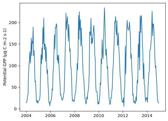
The plot below shows the resulting predictions of mean GPP in µg C m-2 s-1 for each fortnight.
The code below then uses the from_pmodel method to calculate maximum annual fAPAR
using two different methods. Note that method="cai" also requires the additional
variable aridity_index providing estimates of site specific aridity (PET/P), which
should be an array of single climatological values per site, described above.
# Method = "cai", with additional aridity data
faparlim_pmodel_cai = FaparLimitation.from_pmodel(
    method="cai",
    pmodel=pmodel,
    growing_season=fortnightly_data["growing_season"].to_numpy(),
    precip=fortnightly_data["precip_molar"].to_numpy(),
    datetimes=fortnightly_data["time"].to_numpy(),
    aridity_index=np.array([site_data["AI"]]),
)

# Method = "zhu"
faparlim_pmodel_zhu = FaparLimitation.from_pmodel(
    method="zhu",
    pmodel=pmodel,
    growing_season=fortnightly_data["growing_season"].to_numpy(),
    precip=fortnightly_data["precip_molar"].to_numpy(),
    datetimes=fortnightly_data["time"].to_numpy(),
)
/home/docs/checkouts/readthedocs.org/user_builds/pyrealm/checkouts/latest/pyrealm/core/experimental.py:72: ExperimentalFeatureWarning: 'Be aware that FaparLimitation is an experimental feature of pyrealm and the implementation and API may change within major versions.'
  warn(qualname, ExperimentalFeatureWarning)
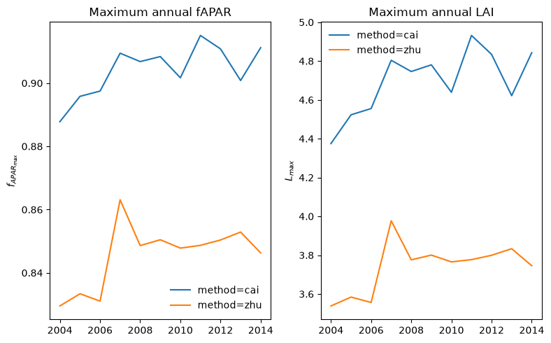
The resulting time series of annual values of \(f_{APAR_{max}}, L_{max}\) are shown below and are basically identical to the calculations from the pre-calculated annual values shown above.
The SubdailyPModel
The code below loads the original half hourly FluxNET data (2004-2014, 192864 values).
# Load subdaily data
subdaily_data_path = get_pyrealm_data("phenology/inputs/subdaily/pmodel_inputs.csv")
subdaily_data = pd.read_csv(subdaily_data_path)
subdaily_data["time"] = pd.to_datetime(subdaily_data["time"])
This dataset is then used to build predictions using the subdaily P Model:
# Calculate the P Model environment
subdaily_pmodel_env = PModelEnvironment(
    tc=subdaily_data["tc"].to_numpy(),
    vpd=subdaily_data["vpd"].to_numpy(),
    patm=subdaily_data["patm"].to_numpy(),
    co2=subdaily_data["co2"].to_numpy(),
    ppfd=subdaily_data["ppfd"].to_numpy(),
    fapar=np.array([1]),
)

# Define the acclimation window for the model
acclim_model = AcclimationModel(datetimes=subdaily_data["time"].to_numpy())
acclim_model.set_window(
    window_center=np.timedelta64(12, "h"), half_width=np.timedelta64(1, "h")
)

# Fit the subdaily P Model
subdaily_pmodel = SubdailyPModel(
    env=subdaily_pmodel_env,
    acclim_model=acclim_model,
)
/home/docs/checkouts/readthedocs.org/user_builds/pyrealm/checkouts/latest/pyrealm/pmodel/pmodel.py:481: UserWarning:
            The default value for quantum yield of photosynthesis (phi0=1/8) has changed
            since pyrealm 1.0.0. You may need to change settings to duplicate results
            from pyrealm 1.0.0.

  warn(
Predicting annual maximum fAPAR is then almost identical to using the standard P Model.
The only difference is that the acclimation model used to fit subdaily P Models already
provides datetimes for each observation, so the datetimes argument is not used:
# Method = "cai", with additional aridity data
faparlim_subdaily_pmodel_cai = FaparLimitation.from_pmodel(
    method="cai",
    pmodel=subdaily_pmodel,
    growing_season=subdaily_data["growing_season"].to_numpy(),
    precip=subdaily_data["precip_molar"].to_numpy(),
    aridity_index=np.array([site_data["AI"]]),
)

# Method = "zhu"
faparlim_subdaily_pmodel_zhu = FaparLimitation.from_pmodel(
    method="zhu",
    pmodel=subdaily_pmodel,
    growing_season=subdaily_data["growing_season"].to_numpy(),
    precip=subdaily_data["precip_molar"].to_numpy(),
)
/home/docs/checkouts/readthedocs.org/user_builds/pyrealm/checkouts/latest/pyrealm/core/experimental.py:72: ExperimentalFeatureWarning: 'Be aware that FaparLimitation is an experimental feature of pyrealm and the implementation and API may change within major versions.'
  warn(qualname, ExperimentalFeatureWarning)
The plots of the annual predicted maximum fAPAR again look very similar.