Estimating acclimation

The worked example from this page can be downloaded as Jupyter notebook here.

Rather than being able to instantaneously adopt optimal values, three key photosynthetic \(\xi\), \(J_{max25}\) and \(V_{cmax25}\) acclimate slowly towards daily optimal values. The modelling approach to representing slow responses within the P Model, following (Mengoli et al., 2022), has three components:

• The identification of a daily window within a set of subdaily observations that defines the optimal daily values for acclimation. This will typically be the set of conditions that maximise daily productivity - the environmental conditions that coincide with peak sunlight.

• The definition of an acclimation process that imposes a lagged response on parameters such that the realised value on a given day reflects previous conditions.

• The interpolation of realised daily values back onto the subdaily timescale.

Show code cell source

Hide code cell source

from copy import copy

import numpy as np
from matplotlib import pyplot as plt
from matplotlib.collections import PatchCollection
from matplotlib.lines import Line2D
from matplotlib.patches import Rectangle, Patch
import matplotlib.dates as mdates

from pyrealm.pmodel.acclimation import AcclimationModel

The acclimation model

Defining the model to be used for estimating acclimation uses the AcclimationModel. This class is used to:

• define the timing of observations on a subdaily scale,

• define an daily acclimation window that sets the daily conditions that plants will optimise their behaviour towards,

• apply acclimation lags to optimal behaviour to give daily realised values, and

• sample daily realised values back to the subdaily time scale.

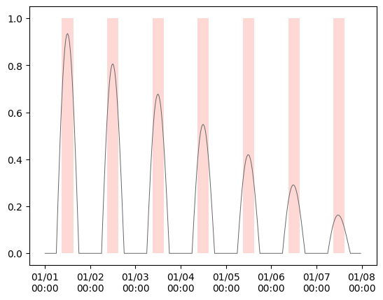
The code below creates a simple time series representing a parameter responding instantaneously to changing environmental conditions on a fast scale.

The code then sets up a AcclimationModel instance using the observations time on the fast scale and sets a 6 hour acclimation window around noon. This is a particularly wide acclimation window, chosen to make it easier to see different approaches to interpolating data back to subdaily timescales. In practice Mengoli et al. (2022) present results using one hour windows around noon or even the single value closest to noon.

# Define a set of observations at a subdaily timescale
subdaily_datetimes = np.arange(
    np.datetime64("1970-01-01"), np.datetime64("1970-01-08"), np.timedelta64(30, "m")
)

# A simple artificial variable showing daily patterns and a temporal trend
subdaily_data = -np.cos((subdaily_datetimes.astype("int")) / ((60 * 24) / (2 * np.pi)))
subdaily_data = subdaily_data * np.linspace(1, 0.1, len(subdaily_data))
subdaily_data = np.where(subdaily_data < 0, 0, subdaily_data)

# Create an acclimation model, using a deliberately wide 6 hour window around noon
acclim_model = AcclimationModel(datetimes=subdaily_datetimes)

window_center = np.timedelta64(12, "h")
half_width = np.timedelta64(3, "h")

acclim_model.set_window(window_center=window_center, half_width=half_width)

The plot below shows the rapidly changing variable and the defined daily acclimation windows.

Show code cell source

Hide code cell source

fig, ax = plt.subplots()

# Add the acclimation windows for each day
acclim_windows = [
    Rectangle(
        (win_center - half_width, 0), 2 * half_width, 1, facecolor="salmon", alpha=0.3
    )
    for win_center in acclim_model.sample_datetimes_mean
]

[ax.add_patch(copy(p)) for p in acclim_windows]

# Show the variable at the subdaily timescale
ax.plot(subdaily_datetimes, subdaily_data, "-", color="0.4", linewidth=0.7)

# Format date axis
myFmt = mdates.DateFormatter("%m/%d\n%H:%M")
ax.xaxis.set_major_formatter(myFmt)

Estimating realised responses

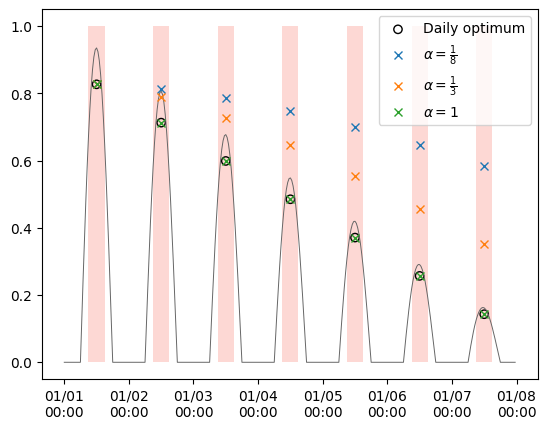
The next step is estimate the daily realised values of slowly responding variables. This is implemented using a rolling weighted average across daily optimal values, following Mengoli et al. (2022). The slow response is calculated as:

\[ R_{t} = R_{t-1}(1 - \alpha) + O_{t} \alpha , \]

where \(O\) is the time series of instantaneous daily optimal values and \(R\) are the realised values incorporating the memory effect, with \(R_{t=0} = O_{t=0}\). The parameter \(\alpha \in (0, 1)\) sets the strength of the memory effect, adjusting the speed with which realised values of these parameters converge on daily optimal values. The value of \(\alpha\) can also be thought of as the reciprocal of the length of the memory window in days (\(d\)), and the default is \(d=15, \alpha=\frac{1}{15}\) for a fortnightly window.

• When \(t < d\), \(R_{t}\) is calculated across fewer actual days of data.

• When \(\alpha = 0\), there is no acclimation: plant responses are fixed at the optimum value for the first day.

• When \(\alpha = 1\), there is no lag and acclimation is instantaneous.

The code below extracts the daily optimal values within the acclimation window and then applies the memory effect with three different values of \(\alpha\). When \(\alpha = 1\), the realised values are identical to the daily optimum value within the acclimation window.

# Extract the optimal values within the daily acclimation windows
daily_mean = acclim_model.get_daily_means(subdaily_data)

# Build acclimation models with different alpha
alpha_models = {}
alpha_vals = (
    (1 / 8, r"$\alpha = \frac{1}{8}$"),
    (1 / 3, r"$\alpha = \frac{1}{3}$"),
    (1, r"$\alpha = 1$"),
)

for alpha, _ in alpha_vals:
    model = AcclimationModel(datetimes=subdaily_datetimes, alpha=alpha)
    model.set_window(window_center=window_center, half_width=half_width)
    alpha_models[alpha] = model

Show code cell source

Hide code cell source

fig, ax = plt.subplots()

# Add the acclimation windows for each day
[ax.add_patch(copy(p)) for p in acclim_windows]

# Show the variable at the fast timescale
ax.plot(subdaily_datetimes, subdaily_data, "-", color="0.4", linewidth=0.7)

# Show the optimal (daily mean) values
ax.scatter(
    acclim_model.sample_datetimes_mean,
    daily_mean,
    facecolor="none",
    edgecolor="k",
    label=r"Daily optimum",
)

# Show the acclimated values under each of the three models
for alpha, label in alpha_vals:
    model = alpha_models[alpha]
    ax.plot(
        acclim_model.sample_datetimes_mean,
        model.apply_acclimation(daily_mean),
        "x",
        label=label,
    )

ax.legend()

# Format date axis
myFmt = mdates.DateFormatter("%m/%d\n%H:%M")
ax.xaxis.set_major_formatter(myFmt)

Interpolation of realised values to subdaily timescales

The realised values calculated above provide daily estimates, but then these values need to be interpolated back to the timescale of the original observations to calculate subdaily predictions. The interpolation process sets two things:

• The update point at which the plant adopts the new realised value.

• The interpolation scheme between one realised value and the next. There are currently two options:

  • The previous option holds the value from the previous acclimation window constant until the update point of the next.

  • The linear option uses linear interpolation between update windows. With this option, the value is held constant for the first day and then applies linear interpolation between the update points. This one day offset in the realised values is always applied to avoid interpolating to a value that is not yet known.

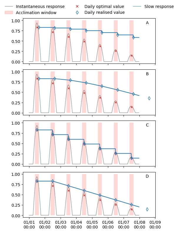
The code below defines four different scenarios for generating realised subdaily values using the fill_daily_to_subdaily() method.

scenarios = {
    "A": dict(alpha=1 / 8, fill_method="previous", update_point="max"),
    "B": dict(alpha=1 / 3, fill_method="linear", update_point="max"),
    "C": dict(alpha=1, fill_method="previous", update_point="mean"),
    "D": dict(alpha=1, fill_method="linear", update_point="mean"),
}

These scenarios are described below and then the results of applying these scenarios on the example data are shown in the plots:

Scenario A

The daily optimal realised value acclimates slowly (\(\alpha = \frac{1}{8}\)) and is held constant from the end (‘maximum’) of one acclimation window until the end of the next.

Scenario B

The daily optimal realised value acclimates more rapidly (\(\alpha = \frac{1}{3}\)) and is linearly interpolated to the subdaily timescale from the end of one acclimation window to the next, after a one day offset is applied. The cross shows the daily realised value and the triangle shows those values with the offset applied.

Scenario C

The daily optimal realised value is able to instantaneously adopt the the daily optimal value in the acclimation window (\(\alpha = 1\)). The realised value at the subdaily scale is held constant from the middle(‘mean’) of one acclimation window until the next.

Scenario D

The daily optimal realised value is again able to instantaneously adopt the daily optimal value, but the one day offset for linear interpolation is applied.

Show code cell source

Hide code cell source

# Create the figure
fig, axes = plt.subplots(4, 1, figsize=(6, 8), sharex=True)

for (scenario_id, scenario_details), axis in zip(scenarios.items(), axes):

    # Add the acclimation windows for each day
    [axis.add_patch(copy(p)) for p in acclim_windows]

    # Get the acclimation model for the scenario
    model = AcclimationModel(subdaily_datetimes, **scenario_details)
    model.set_window(window_center=window_center, half_width=half_width)

    # Get the daily optimal values within the window, apply acclimation
    # to get the daily realised values and then fill back onto the subdaily
    # scale, using the return_interpolation_inputs option to get the
    # inputs to the interpolation process
    daily_optimal = model.get_daily_means(subdaily_data)
    daily_realised = model.apply_acclimation(daily_mean)
    interp_x, interp_y, _ = model._get_subdaily_interpolation_xy(daily_realised)
    subdaily_realised = model.fill_daily_to_subdaily(daily_realised)

    # Show the variable at the subdaily timescale and the daily optimal values
    axis.plot(subdaily_datetimes, subdaily_data, "-", color="0.4", linewidth=0.7)
    axis.scatter(
        model.sample_datetimes_mean,
        daily_optimal,
        s=15,
        c="C3",
        marker="x",
        linewidth=1,
    )

    # Add the filled subdaily values, along with the interpolation inputs, showing
    # the realised daily values at the point at which the interpolation values update.
    axis.plot(model.datetimes, subdaily_realised)
    axis.scatter(
        interp_x,
        interp_y,
        marker="d",
        edgecolor="C0",
        facecolor="none",
    )

    # Add a scenario label
    axis.text(0.95, 0.95, scenario_id, ha="right", va="top", transform=axis.transAxes)

    # Format date axis
    myFmt = mdates.DateFormatter("%m/%d\n%H:%M")
    axis.xaxis.set_major_formatter(myFmt)

# Add a shared legend
axes[0].legend(
    loc="lower center",
    bbox_to_anchor=[0.5, 1],
    ncols=3,
    frameon=False,
    handles=[
        Line2D([0], [0], label="Instantaneous response", color="0.4", linewidth=0.7),
        Patch(color="salmon", alpha=0.3, label="Acclimation window"),
        Line2D(
            [0],
            [0],
            label="Daily optimal value",
            color="C3",
            linestyle="none",
            marker="x",
        ),
        Line2D(
            [0],
            [0],
            label="Daily realised value",
            markeredgecolor="C0",
            linestyle="none",
            marker="d",
            markerfacecolor="none",
        ),
        Line2D([0], [0], label="Slow response", color="C0", linewidth=0.7),
    ],
)
plt.tight_layout()